SixTrack: tracking particles and post-processing long-term stability data
This article is part of a short series adapted from my Bachelor's thesis on post-processing routines for long-term beam stability in particle accelerators.
The previous article in this series laid out the coordinate systems, Hamiltonian mechanics and beam optics used to describe a particle's motion in an accelerator. This one introduces SixTrack, the particle-tracking code that actually puts that theory to work for the LHC, describes the problems it's built to tackle, and walks through its post-processing subroutine — the part of the code this whole series is ultimately about documenting, and eventually porting to Python.
1. Particle Tracking#
Particle tracking has become a key tool for the simulation and study of beam behaviour inside an accelerator. We use it for, among other things, calculating and predicting the dynamic aperture (the effective aperture of the particle motion) and its dependence on non-linearities and tunes, finding closed-orbit distortions, or assessing the long-term stability of the beam.
Over the past thirty years, simulation codes like SixTrack, MAD-X, RACETRACK1 or PTC have been developed to apply particle-tracking techniques from different angles. These codes simulate the movement of a particle inside the high-energy ring for thousands of turns, observing its characteristics — amplitude, phase advance, coordinates — at the same position s₀ on every one of those turns.
Tracking codes have traditionally struggled with rounding precision and limited CPU time. Processing time has steadily improved, helped along by distributed-computing efforts like the CPSS project and the LHC@Home platform we met in the previous article, but the problem of rounding-related differences between platforms persisted for every available compiler until SixTrack finally solved it by including the crlibm library, which corrects rounding-error differences in a portable way, together with strict ordering of operations and specific compiler flags — making the result numerically reproducible across machines.
A typical SixTrack dynamic-aperture study for the LHC involves simulating 5 different angles in phase-space and 60 different representations of the magnetic errors (seeds), tracking 30 pairs of particles for 10⁵ turns in each case. A study of that size can take several days, since each individual case needs around 2 hours of computing time to finish.
2. SixTrack#
SixTrack2 is a single-particle, six-dimensional symplectic tracking code optimized for long-term tracking in high-energy rings. Based on RACETRACK and first published in 1990 by Frank Schmidt, it has been used for several kinds of LHC studies: dynamic aperture, tune optimization, collimation studies, and more. SixTrack has been under heavy development for the past 25 years3, and keeps evolving with improvements like the database-based post-processing port this series covers, new physics models, new particle parameters (mass, charge state), and GPU libraries to offload the computationally heavy parts.
SixTrack is written in Fortran 77 and comes to more than 70,000 lines of code, in a structure that requires a pre-processor to simplify the code and substitute special expressions in the source files, applying the Differential Algebra extension for Fortran (DAFOR). Figure 1 shows the shape of this build process.
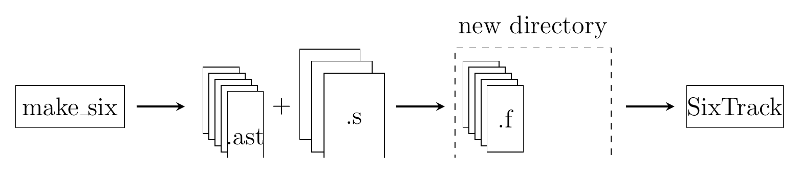
Figure 1: SixTrack build process. The make_six script generates an .ast mask file for each Fortran file to be produced; these masks select the blocks of code from three .s source files (sixtrack.s, lielib.s and dabnew.s) that end up in the final Fortran files, which are then linked and compiled into the SixTrack executable.
Running make_six generates five Fortran files: track.f, containing the tracking maps for every lattice element (dipoles, quadrupoles, octupoles, RF cavities, higher-order magnets, crab cavities); sixve.f, the main file, defining the main program, most subroutines, and the postpr post-processing subroutine this article is mostly about; sixvefox.f, containing the subroutines for the closed-orbit and lattice-optics mapping, using a differential-algebra approach; lielib.f, E. Forest's subroutines for normal-form calculations; and dabnews.f, the DAFOR subroutines called by sixvefox.f during the closed-orbit calculation.
These files are compiled into a single Fortran executable, which takes as input the description of the accelerator in the fort.2 file and the settings and description of the elements in the fort.3 file. It then initializes all parameters and variables, computes the six-dimensional closed orbit together with the Courant-Snyder invariants introduced in the previous article, and performs the tracking. Finally, the tracking data is analyzed and post-processed as specified in fort.3.
3. SixTrack's Post-Processing: A Walkthrough#
The postpr subroutine is SixTrack's post-processing engine. It reads the binary tracking output — one record per turn, per particle pair, written to the fort.10 file in a fixed, documented binary layout — and reduces thousands of turns of raw six-dimensional coordinates down to a handful of physically meaningful numbers per angle and seed: an estimate of the dynamic aperture, a measure of how non-linear the motion really was, and how many turns each particle pair actually survived before being lost. None of that mapping — which Fortran variable corresponds to which physical quantity, and which formula from the previous article each block of code is actually evaluating — came with the code or with the papers it cites; working it out, variable by variable, against the beam-optics formulas is what makes the rest of this section possible. The description below covers the overall shape of that process and a few of its more interesting steps; the implementation details reflect SixTrack as it stood around 2015-16, and parts of it may well have evolved since.
After opening the binary file, postpr first reads its header: the number of particle pairs and turns to expect, the closed orbit and dispersion vectors, and the one-turn transfer matrix (and its inverse) at the observation point, all of which the rest of the subroutine will need to compute deviations and invariants correctly for this particular study.
After reading the file's header and initializing its parameters, the very first thing postpr does with the actual tracking data is call a subroutine called distance, which computes the separation, in phase-space, between a particle and its "twin" — a second particle launched from an almost identical initial condition. SixTrack always tracks particles in such close-by pairs for exactly this reason: as long as the motion is linear, two initially close-by particles stay close together turn after turn, but as soon as non-linear effects become significant their separation starts to grow, and tracking how fast it grows (essentially estimating a Lyapunov exponent) is one of the main ways SixTrack detects the onset of chaotic motion — and with it, the dynamic aperture.
From there, postpr computes the deviation of each particle's coordinates from the closed orbit — what the code calls c, d, e, f and the Fortran source denotes \(\tilde{x}, \tilde{x}', \tilde{y}, \tilde{y}'\) — and feeds them into two lines that, on their own, look like unremarkable Fortran arithmetic:
xp0 = bet0(1)*d + alf0(1)*c
emx = (c**2 + xp0**2) / bet0(1)
Matched up against the beam-optics formulas from the previous article — none of which appear anywhere in SixTrack's source or comments — these two lines turn out to be exactly the Courant-Snyder invariant for the horizontal plane:
\[ xp_0=\beta_{xI}\tilde{x}'+\alpha_{xI}\tilde{x}, \qquad \epsilon_x=\frac{\tilde{x}^2+(\beta_{xI}\tilde{x}'+\alpha_{xI}\tilde{x})^2}{\beta_{xI}}, \]with bet0(1) and alf0(1) holding the horizontal \(\beta_{xI}\) and \(\alpha_{xI}\) lattice functions computed earlier in the run. The vertical emittance \(\epsilon_y\) follows the identical pattern one plane over, and the combined transverse emittance is simply \(\epsilon_{vt}=\epsilon_x+\epsilon_y\). postpr keeps running maximum, minimum and average values of each of these three emittances as it goes, together with the averaged phase advances.
From the evolution of these emittances, postpr computes one of its more interesting diagnostics: the smear, essentially the normalized variance of the emittance around its running average, expressed as a percentage. Under purely linear motion the invariant stays constant turn after turn, so its smear is zero; non-linear perturbations make it wobble, and the size of that wobble is a direct, quantitative measure of how non-linear the particle's motion actually is at a given amplitude. SixTrack computes it both for the horizontal and vertical planes separately and for the combined transverse motion, fitting its evolution with two separate fitting functions to smooth out the turn-by-turn noise before reporting a single representative value.
None of these numbers is very informative in isolation — what actually matters for a dynamic-aperture study is how the smear, the survival turns and the other diagnostics behave as a function of the amplitude at which a given pair of particles was launched, repeated over several angles in phase-space and several seeds representing different realizations of the machine's magnetic errors. A single SixTrack run only produces the numbers for one such angle and seed; it's only once postpr's output from every run in a study gets collected and compared side by side that a clear picture of the dynamic aperture — the largest amplitude at which motion remains reliably stable — starts to emerge. That collection step is itself a form of post-processing, and it's the one SixDesk is responsible for.
Finally, postpr keeps track of how many turns each particle pair survives before either one is lost (typically once its amplitude grows past a cut-off) — the survival count — and fits the evolution of the distance between twin particles to extract a maximum slope, a more direct estimate of how quickly chaotic motion is setting in at that angle. Once all the available turns and particle pairs have been processed, postpr prints one summary record per angle and seed — covering the average emittance, the smear, the survival turns and the maximum slope among others — and, optionally, hands the same numbers off to a set of GNUPlot scripts to produce plots of these quantities directly from the Fortran run.
4. From SixTrack to SixDesk's Post-Processing#
SixDesk, the run environment for SixTrack introduced in the previous article, takes the results of a SixTrack study and applies its own post-processing layer on top.
By default, SixDesk's scripts automatically tar all of a SixTrack run's output files and store them in CASTOR4, CERN's hierarchical mass-storage system. Among these tars is fort.6, which logs every operation performed and any failures that may have occurred during the run, and a set of binary files, fort.90 down to fort.59, used for further analysis and documented in SixTrack's own manual5.
As for the main output file, fort.10: running the run_join10 script gathers the results of all the completed jobs of a study and combines their output files. Once combined, the fort.10 data can be post-processed to find the chaotic boundary and the particle losses described above, across an entire study rather than a single run.
SixDesk also provides a couple of options for plotting, controlled by two sixdeskenv variables: if iplot is set, a plot is produced for every seed (which can generate a very large amount of data, even compressed); and kvar, which, left at its default, produces the dynamic aperture as a function of angle, both per seed and averaged over all seeds — an extremely time-consuming procedure, but one of the most direct ways to visualize a study's overall result.
That combination — a 70,000-line Fortran codebase, binary files tarred away into mass storage, and a pair of environment-variable flags controlling whether a multi-day plotting pass runs or not — is exactly the shape of the problem the next and final article in this series sets out to fix, by porting this whole post-processing pipeline to a Python- and SQL-backed implementation: SixDeskDB.
-
Wrulich, A. (1984). RACETRACK—a computer code for the simulation of nonlinear particle motion in accelerators. ↩︎
-
Schmidt, F. (1990). Sixtrack. CM-P00049314. ↩︎
-
De Maria, R., Previtali, V., Levinsen, Y., Lari, L., Schmidt, F., Renshall, H., Barranco, J., Mereghetti, A., Appleby, R., Vlachoudis, V., et al. (2013). Recent developments and future plans for SixTrack. ↩︎
-
Presti, G. L., Barring, O., Earl, A., Rioja, R. M. G., Ponce, S., Taurelli, G., Waldron, D., & Dos Santos, M. C. (2007). CASTOR: A Distributed Storage Resource Facility for High Performance Data Processing at CERN. MSST, 7, 275-280. ↩︎
-
Schmidt, F. (1994). SixTrack, User's Reference Manual. CERN SL/94-56 (AP). ↩︎