Porting SixDesk's post-processing to Python and SQL
This article is part of a short series adapted from my Bachelor's thesis on post-processing routines for long-term beam stability in particle accelerators. Some of the implementation details below reflect SixDesk/SixDeskDB as they stood in 2015-16 and may not match their current state.
The previous article in this series walked through postpr, SixTrack's Fortran post-processing subroutine, and the pile of interdependent Bash, AWK and Fortran scripts SixDesk wraps around it to turn a full dynamic-aperture study into a handful of plots. This last article in the series covers the actual engineering contribution of the thesis: porting that whole pipeline to a database-centered Python and SQL implementation, SixDeskDB.
1. SixDeskDB: SixDesk's Database Port#
During 2014, and especially over the summer with the help of students provided by Google Summer of Code, a database-centered Python port of SixDesk was developed. Using a database approach has several benefits:
Reduces complexity: it replaces a design made of several interdependent Bash, AWK, GNUPlot and Fortran scripts with a Python implementation that uses SQL for queries.
Solves AFS's limitations: AFS can hold, at most, around two thousand entries in a single directory, but longer SixTrack simulations demand far more entries than that for all the files they generate. Using a database as the file and data server removes this limitation entirely.
No need to know Fortran: it's implemented in Python and SQL, both less complex, more flexible and far more widely used than Fortran.
Improves execution times: removing all the operations that require writing a huge amount of files to disk dramatically improves execution time.
Introduces object-oriented programming, with its benefits (and trade-offs) applied to SixTrack.
Adds flexibility: generating every file and plot into a rigid filesystem tree is no longer required; they can instead be produced on request, which makes them easier to manipulate and leaves more room to extend or change the code later.
Allows the use of modern, popular, state-of-the-art scientific libraries: NumPy and SciPy can be used without as much of a performance hit as one might expect from replacing Fortran with an interpreted language.
On the other hand, it does add a new language to the stack needed to work with SixTrack, and it will eventually require its own adaptation for use with the LHC@Home platform.
2. The Post-Processing Run#
SixDesk's post-processing run makes use of several interdependent Bash, AWK, GNUPlot and Fortran scripts, alongside a series of configuration files and SixTrack's own tracking output files.
The main script to run is run_post, after run_join10 and run_awk have prepared, on request, the files it takes as input: run_join10 combines all the individual fort.10 files from a study into a single joint file (the same joining step the previous article described), and run_awk takes that joint file and parses it into the intermediate files the plotting step needs. The important functions actually called during the post-processing run are read10b and readplotb, where the core post-processing calculations happen — these are the two Fortran functions SixDeskDB needs to port, together with the management and looping currently spread across several Bash scripts around them.
After the post-processing run, the results come out in a file tree structure like the one in Figure 1, with some of the binary output files carrying further information about the process also stored automatically in CASTOR1.
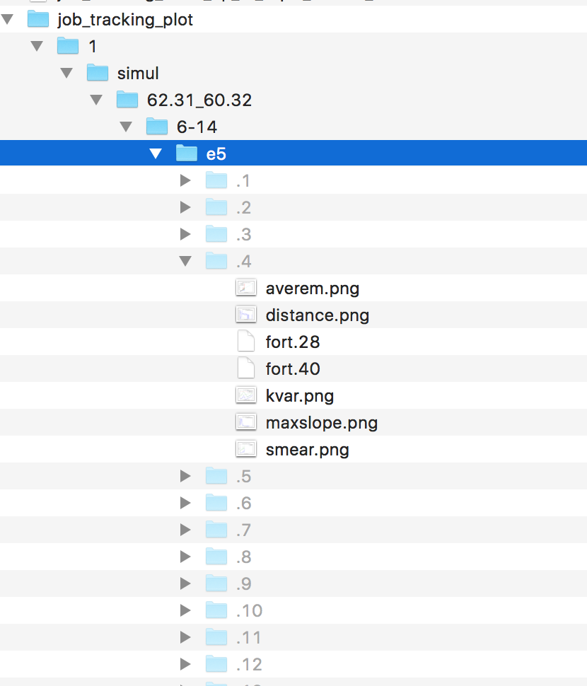
Figure 1: SixDesk's output file tree for a long run. The output files are generated along a path following the structure /<seed>/simul/<tune range>/<amplitude range>/<order of the number of turns>/<angle>/outputFiles.
It's worth noting how quickly a typical SixTrack DA study for the LHC — 5 angles in phase-space across 60 seeds — exceeds AFS's directory-entry limitations, and how long it takes to compute and write to disk this way. Hence the need for a new implementation.
3. Design and Implementation#
The code developed aims to fully reproduce the physics side of SixDesk's post-processing run — the code in the read10b and readplotb Fortran files, together with the Bash scripts that launch and loop over them. That means performing dynamic-aperture analysis, finding particle losses and chaotic boundaries, and so on. The first design decision was to move this analysis out of SixDeskDB's main class entirely, into a class of its own, rethinking the software architecture around it. (At the time of writing, this is still an unfinished project — everything described here reflects its state at this particular moment.)
Figure 2 shows a simplified dependency diagram for the classes involved.
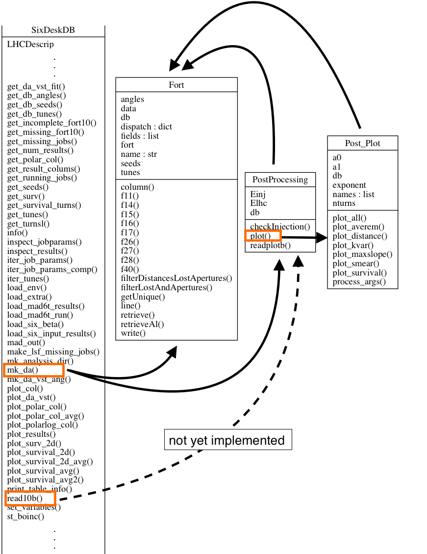
Figure 2: Dependencies between classes and functions in this project's implementation of the post-processing run.
There are a few interesting things to note about how these classes work together:
SixDeskDB: SixDesk's main Python class. It does almost everything SixDesk can do, and although at this stage its role isn't to perform every operation itself, it's in charge of reading the input files, OS and file management, and serving as the interface users call to run each of SixDesk's modules and analyses. This project adds themk_dafunction (short for "make dynamic aperture analysis"), which invokes the post-processing run; theread10bfunction still remains to be ported from this class intoPostProcessing.Fort: a new, auxiliary class that serves as an interface to retrieve the variousfortfiles from the database, hiding the SQL queries from the physics code — and even fromFortitself, since they're defined separately inqueries.py— and giving a more intuitive way to explore the data: every field in everyfortfile is named, for easy access, filtering and manipulation. This way of working with the database is already fully integrated intoPostProcessingandPost_Plot, and is making its way intoSixDeskDBitself.PostProcessing: the class in charge of the physics computations and of generating the output/resultsfortfiles. It currently implements SixDesk'sreadplotbfunction.Post_Plot: the plotting class. It defines the mechanisms needed to generate plots (for long runs only, at the moment) and answersPostProcessing'splot()call.
This structure adds another layer of complexity to SixDeskDB, but in return it brings a few real advantages: Fort files on request, since the Fort class can retrieve any generated Fort file on request, indexed by angle and seed, without writing redundant files to disk, and can even recover intermediate post-processing files that the original run_post discarded; plots on request instead of generating every plot during the run, cutting out a lot of unnecessary work; clarity, since Python's mandatory indentation and object-oriented style, combined with using a single language to code in (and SQL to query), make the code far easier to structure, maintain and understand than the original scripts; easily modifiable queries, since keeping the queries that retrieve and generate fort-file data in one separate file makes them faster to change and easier to extend with new ones; and control over the output, since the Fort class exposes the same data SixDesk's Fortran code generates, structured the same way, with useful extras like indexing by variable layered on top.
Table 1 lists the output fort files this implementation reproduces and the columns tracked in each; Table 2 describes what each of those columns actually means.
| File | Columns |
|---|---|
fort.11 | achaos, al, amin, amax, achaos1 |
fort.12 | rad, distp |
fort.13 | rad, dist |
fort.14 | achaos, alost3, turn_max, f14 |
fort.15 | rad, sturns1, sturns2 |
fort.16 | deltap, qx, qy |
fort.17 | deltap, qx, qy |
fort.18 | rad, smearx |
fort.19 | rad, smeary |
fort.20 | rad, qx_det |
fort.21 | rad, qy_det |
fort.22 | rad, rad1*sigxminnld |
fort.23 | rad, rad1*sigxavgnld |
fort.24 | rad, rad1*sigxmaxnld |
fort.25 | qx_det, qy_det, qx_det+qx, qy_det+qy |
fort.26 | achaos, alost2, amax |
fort.27 | al |
fort.28 | al |
fort.40 | achaos, al, amin, amax |
Table 1: Reference table for the output fort files and the variables tracked in them.
| Column | Description |
|---|---|
achaos | the chaotic boundary, with the slope method |
achaos1 | distance in phase-space, with the slope method |
al | aperture lost |
amin | minimum aperture |
amax | maximum aperture |
rad | ratio εI/ε (or εII/ε), where ε = εI² + εII², normalized to the user-specified beam emittance |
rad1 | the same quantity as rad, but evaluated using the average amplitudes and secondary beta functions |
dist | distance in phase-space |
distp | maximum slope of the distance in phase-space |
alost1 | average, corrected initial condition of a lost particle |
alost2 | initial condition of a lost particle |
turn_max | maximum number of turns |
sturns1, sturns2 | survived turns of the first and second particle of the pair |
deltap | relative momentum deviation |
qx, qy | horizontal and vertical tune |
qx_det, qy_det | horizontal and vertical detuning |
smearx, smeary | horizontal and vertical smear |
Table 2: Output fort files' column names (variables) reference.
4. Results and Plotting#
All results produced by this implementation have been checked to match the originals to a precision of ten decimal places — more than enough, considering the values are stored as strings in the database.
Alongside the numerical results, a plotting module was developed to replace the entangled web of Bash and AWK scripts that made up SixDesk's original plotting functionality, built on Matplotlib instead of GNUPlot. Every long-run plot has been reproduced and matches its original, which is itself a useful cross-check of the results. One caveat: because of a bug in the version of Matplotlib paired with the NumPy version used at CERN at the time, logarithmic axis scales couldn't be used in the new plots — which is why, in the comparison below, the new survival-time plot uses a linear y-axis where the original used a logarithmic one.
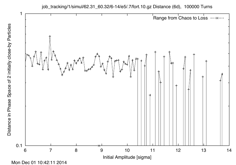
SixDesk (original)
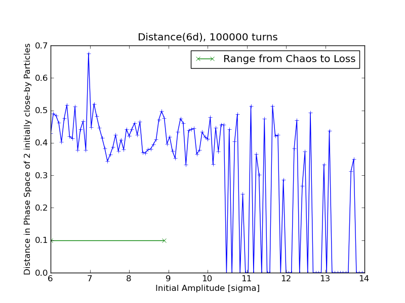
SixDeskDB (ported)
Figure 3: Distance in phase-space of two initially close-by particles — the end value of d(turns) as a function of initial amplitude, for seed 1, angle 7 — reproduced in SixDeskDB (bottom) against SixDesk's original GNUPlot output (top).
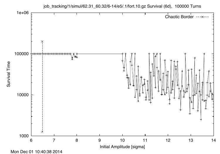
SixDesk (original)
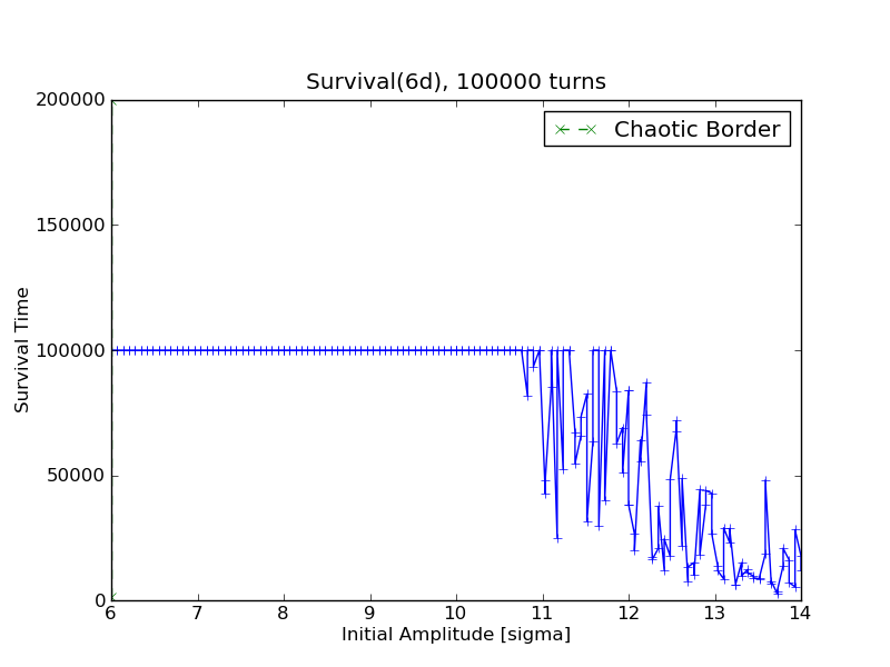
SixDeskDB (ported)
Figure 4: Survival time versus initial amplitude, for seed 1, angle 1 — SixDeskDB's version (bottom) against the original (top); note the linear instead of logarithmic y-axis, for the Matplotlib reason mentioned above.
5. Conclusions#
Post-processing is the key feature of SixDesk, and one of the core parts of SixTrack. Documenting it thoroughly — precisely enough to trace what SixTrack is doing at each step of the post-processing — matters in its own right: the original authors of this code were, for a long time, the only people who really understood how it worked, and they stopped actively working on the project around a decade ago. Beyond the code itself, what was needed most was an adaptation of the theoretical foundations — mostly worked out in 4D in the literature — to the full 6D phase-space SixTrack actually works in; getting there meant carefully inspecting the Fortran code and its program flow and cross-checking the results against the 4D derivations and the theory this series opened with.
SixDeskDB takes that documented understanding and turns it into a modern, modular, widely-used and clear implementation in Python. Since Python is one of the most used languages at CERN, this port opens up the development of new SixDesk analyses to a much wider audience than the original Fortran and Bash ever could, and it brings SixDeskDB a step closer to being able to fully replace SixDesk itself — now faster to develop against, more efficient with disk space, quicker to execute, and augmented with features like fetching plots and Fort files on request through a friendly interface that hides the SQL behind it.
There's plenty of work still ahead: post-processing short runs and integrating them into the program flow; refactoring readplotb to share more of its code with the new read10b; integrating the Fort class more fully across the rest of SixDeskDB; documenting SixDeskDB's own variables independently of SixDesk's; and, further out, new physics models, integration with the LHC@Home platform, consolidating the various homegrown forks of SixTrack, and improving the precision and use of floating-point arithmetic throughout.
This wraps up this short series — from the beam dynamics and particle tracking theory it all rests on, through SixTrack's own Fortran post-processing, to this Python and SQL port of it. If you'd like to go back to the start, the first article is Particle tracking and beam dynamics in accelerators.
-
Presti, G. L., Barring, O., Earl, A., Rioja, R. M. G., Ponce, S., Taurelli, G., Waldron, D., & Dos Santos, M. C. (2007). CASTOR: A Distributed Storage Resource Facility for High Performance Data Processing at CERN. MSST, 7, 275-280. ↩︎