Particle tracking and beam dynamics in accelerators
This article is part of a short series adapted from my Bachelor's thesis on post-processing routines for long-term beam stability in particle accelerators.
Accelerators have become a key tool for the study of experimental particle physics. Today, thousands of physicists around the world depend on the results generated by the Large Hadron Collider.
Having such a large number of people relying on the results of one of the most complex pieces of engineering ever built demands extraordinary precision in the computation and tuning of the path the beam will follow. Simulators like SixTrack exist precisely for that purpose.
This article introduces CERN as an accelerator complex, explains what we hope to achieve by tracking particles, and lays out the theoretical foundations — the coordinate systems, Hamiltonian mechanics and beam optics — that the rest of this short series builds on.
That last part is worth a word of its own. SixTrack's underlying physics had traditionally gone undocumented, and the handful of papers it was originally based on only worked things out in four dimensions, covering part of the six-dimensional formulation its post-processing actually needs. There was no reference anywhere that mapped the code directly to the physics it was meant to implement. Section 6 below is the result of reconstructing that mapping: working backward from SixTrack's Fortran, matching each computed quantity to the formula it was supposed to correspond to, and cross-checking the result against whatever four-dimensional derivations existed in the literature until the two actually lined up. The payoff of that reconstruction shows up directly in the next article, where it's what lets us say, with real confidence, exactly which formula each line of SixTrack's post-processing subroutine is computing.
1. CERN#
A particle accelerator is a machine built out of a large number of magnets and electromagnetic devices. These devices are the ones in charge of guiding the beam through the path described by the accelerator.
CERN is a complex of accelerators created as an intergovernmental organization in 1954 to spark the study of particle physics, making use of the several linear and circular accelerators built with the collaboration of its member and associate member states.
Not all accelerators are equal or serve the same purpose. At CERN, linear accelerators (LINAC2, LINAC3) are mainly used to inject the beam into the circular ones, and some of these circular accelerators require a previous pass through other, smaller circular accelerators just to make sure the beam is injected at the right speed.
There are two beams at a time circulating on this chain of accelerators, each consisting of a large number of bunches of the order of 1011 protons. For the Large Hadron Collider (LHC), the chain starts by extracting protons from hydrogen gas and injecting them into LINAC2. LINAC2 accelerates the protons to 50 MeV and then injects them into the PS Booster, which brings them up to 1.4 GeV. Both beams are then injected into the PS (Proton Synchrotron) and accelerated to 25 GeV, before being passed to the last link of the chain — and the second biggest accelerator at CERN — the SPS (Super Proton Synchrotron), where they reach the required injection energy for the LHC, 450 GeV. Finally, in the LHC, the beams are accelerated up to 7 TeV of energy.
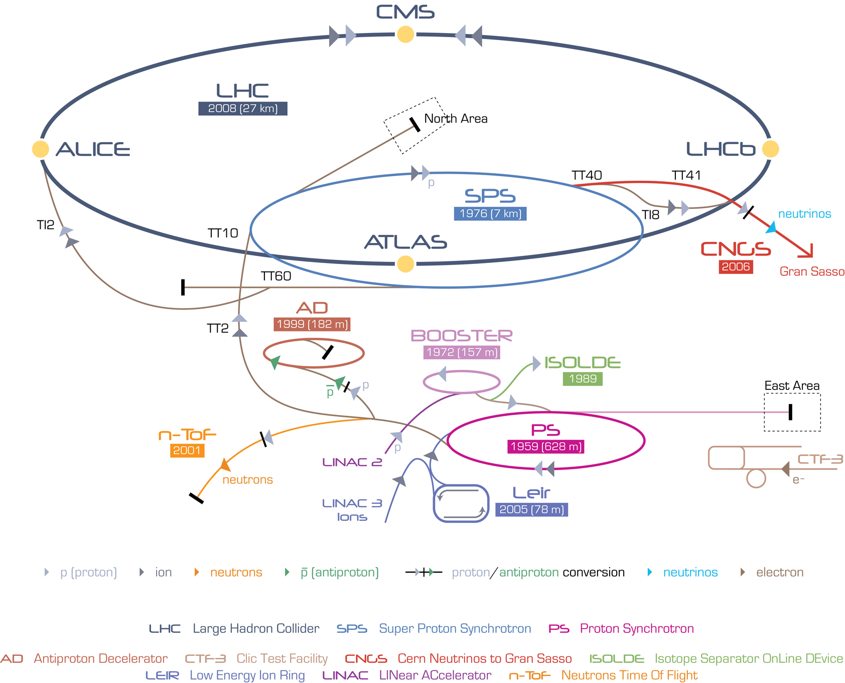
Figure 1: The CERN accelerator complex, including the LHC chain. The yellow dots in the LHC represent each one of the four big experiments.
At CERN, particle physics is studied in several ways, with the study of optics and beam dynamics being one of its most central parts. This is done, for instance, by tracking particles in the beam and observing them at the same point of the synchrotron on every turn.
2. Beam Dynamics and Particle Tracking#
Most of the effects of beam dynamics in an accelerator can be observed by tracking a single particle, rather than a whole bunch of them, inside an electromagnetic field that represents the combination of the diverse elements that make up the accelerator: dipoles, quadrupoles, drift spaces, and so on.
We can define the equations of motion for each one of these devices and simplify them into a one-turn symplectic matrix, making good use of the properties of Hamiltonians to describe the electromagnetic field of the circular accelerator.
Particle tracking is useful, for example, for studying the dynamic aperture or the long-term stability of the beam, and because of this, particle tracking codes aimed at different studies, configurations and accelerators started to appear. One of the longest-lived of these is SixTrack.
3. SixTrack and the LHC@Home Platform#
Accelerators are incredibly complex machines that require a huge amount of energy and time to run, and the slightest deviation in the calculation of the optics or the energy needed — or even a setup error, such as not achieving the required vacuum, a loose screw, or millimeters of difference between the platforms it stands on — can cause months of delay to its operation.
At the same time, the energy required and produced, together with the limitations of what the materials can withstand, mean that the LHC can only be operated during a limited amount of time. This forces physicists to select, from all the tests they would ideally like to run given infinite time, the ones they can actually afford within a fixed time window, and to tune the beam as precisely as they can to get the results they are after.
In this context, simulation codes become an essential tool. SixTrack1 is a six-dimensional, single-particle tracking code aimed at analyzing single-particle effects in circular accelerators.
As mentioned above, accelerators are complex enough that even simulators like SixTrack depend heavily on the flexibility of the parameters used to tune the simulations and studies run on them. This flexibility makes the tool powerful, but also hard to use. For the sake of simplicity, a run environment for SixTrack called SixDesk2 was developed, hiding most of the complications: users only need to tune the parameters in a specific file that is parsed and fed into SixTrack to run a study.
But as technology advanced, other bottlenecks appeared. The construction of new, bigger and more complex accelerators, together with the continuous growth of computer-aided research, fueled a scientific advance never seen before. Soon the processing power of traditional computers was not enough for the biggest simulations, and the demand for more computational power kept growing.
This search for more computational power led to the implementation of the LHC@Home platform3: a volunteer computing system for massive numerical simulations of beam dynamics and high-energy physics events, where volunteers from all around the world — currently more than 125,000 registered users — help run beam dynamics simulations by contributing the spare processing capacity of their home and laptop computers. SixTrack was the first project at CERN to make use of distributed computing this way, achieving a ten-to-hundredfold increase in computing capacity by implementing and making use of the BOINC4 libraries, which split the work into binaries and send each piece to volunteer computers for execution whenever they are idle.
SixTrack and SixDesk's own code, on the other hand, is a complex mixture of Fortran 77, C and various shell scripts and utilities — SixTrack's core alone is more than 70,000 lines of Fortran code, managed by a preprocessor. The growth fueled by LHC@Home has pushed this code to its limits in more mundane ways too: the number of files these studies generate has repeatedly hit the maximum-entries-per-folder limit of AFS, the distributed file system used at CERN. Motivated by that, and by the fact that the underlying physics of SixTrack's post-processing routines has traditionally been under-documented5, a database-centered Python port of SixDesk's post-processing was started — which is exactly what the rest of this short series is about: walking through SixTrack's existing Fortran post-processing, and then porting it to Python and SQL.
4. Coordinate System#
While describing the motion of a particle inside an accelerator, it is convenient to carry out a change of coordinates to a Frenet-Serret coordinate system, like the one shown in Figure 2.
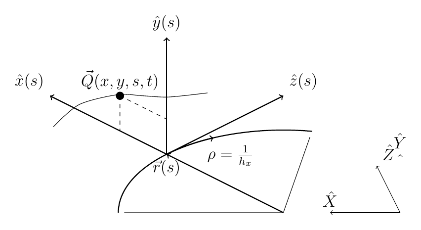
Figure 2: Moving reference frame with its horizontal, vertical and longitudinal axes, parameterized by s(t). The trajectory of a particle Q can be described by the coordinates (x, y, s, t).
This coordinate system moves with the particle along a reference trajectory defined by an ideal particle. This trajectory, the design orbit, represents the ideal closed orbit that a reference particle with constant energy follows in a uniform and constant magnetic field — meaning an ideal particle would circulate in the machine forever.
Assuming the design orbit exists, it is referenced in Figure 2 by \(\vec{r}_0(s)\), where the path length \(s\) measures the distance to a chosen origin along the design orbit. This path is described by \(\vec{Q}(x,y,s,t)\), where \(x\) and \(y\) are the transverse coordinates relative to the design orbit.
Along this ideal orbit, the bending radius \(\rho(s)\) and its inverse \(h(s)\) remain constant; we denote the inverse bending radius as \(h_x\) or \(h_y\) depending on the plane in which the bending happens.
To describe the trajectory of the particle relative to the design orbit, three unit vectors are used: the tangent vector \(\vec{e}_s\), the unit normal vector \(\vec{e}_N\), and the unit binormal vector \(\vec{e}_B\). It is however convenient to define two new unit vectors combining the last two:
\[ \vec{e}_x(s)=\begin{cases} +\vec{e}_N(s), & \text{orbit in horizontal plane}\\ -\vec{e}_B(s), & \text{orbit in vertical plane} \end{cases} \] \[ \vec{e}_y(s)=\begin{cases} +\vec{e}_N(s), & \text{orbit in horizontal plane}\\ +\vec{e}_B(s), & \text{orbit in vertical plane} \end{cases} \]which leads to \(\vec{e}_x(s) \times \vec{e}_y(s) = \vec{e}_s(s)\), meaning \(\{\vec{e}_x(s), \vec{e}_y(s), \vec{e}_s(s)\}\) form a right-handed orthonormal system, with \(\vec{e}_x(s)\) always in the horizontal plane and \(\vec{e}_y(s)\) always in the vertical one. With that, the equation of motion of the tracked particle becomes
\[ \vec{Q}(x,y,s,t)=\vec{r}_0(s(t))+x\cdot \vec{e}_x(s(t))+y \cdot \vec{e}_y(s(t)) \]5. Hamiltonian Mechanics#
In accelerator physics, three alternate approaches to classical mechanics are used: Newtonian, Lagrangian and Hamiltonian mechanics. They differ in the way they define a dynamical system in its canonical form — using the force, the Lagrangian, or the Hamiltonian, respectively.
Conventional, classic Newtonian mechanics can be summarized with the equation
\[ \sum_i F_i = \frac{d(mv)}{dt}, \]which relates the sum of the forces of a system to the temporal evolution of its mechanical momentum.
In the Lagrangian mechanics approach, the Lagrangian \(L\) of a system is defined as
\[ L \equiv T - V, \]where \(T\) is the kinetic energy of the system and \(V\) is its potential energy. Given the Lagrangian as the function \(L(q_j, \dot{q}_j, t)\), the equations of motion of the system can be expressed as
\[ \frac{d}{dt}\left(\frac{\partial L}{\partial \dot q_j}\right) - \frac{\partial L}{\partial q_j} = 0, \qquad (j=1,\ldots,n), \]where qi are the components of q. This formulation is known as the Euler-Lagrange equations of motion.
The third formulation, Hamiltonian mechanics, is the one used for the rest of this project. From the same Lagrangian \(L(q_j, \dot q_j, t)\), the conjugate momenta \(p_i\) of the system can be obtained by
\[ p_i \equiv \frac{\partial L(q_j, \dot q_j, t)}{\partial \dot q_i}, \qquad i=1,\ldots,n. \]The Hamiltonian of a system is defined in terms of a set of coordinates qi and their corresponding momenta pi — these coordinate pairs \((q_i, p_i)\) are known as canonical variables, and the Hamiltonian is written
\[ H=\sum_i \dot q_i p_i - L(q, \dot q, t). \]If the forces acting on the system are conservative and the position in space does not explicitly depend on time, the Hamiltonian follows
\[ H = T + V, \]i.e. it is an expression for the total energy of the system. Given the Hamiltonian, the equations of motion for the dynamical system can then be expressed as
\[ \frac{dx}{dt} = +\frac{\partial H}{\partial p_x}, \quad \frac{dy}{dt} = +\frac{\partial H}{\partial p_y}, \quad \frac{dz}{dt} = +\frac{\partial H}{\partial p_z}, \] \[ \frac{dp_x}{dt} = -\frac{\partial H}{\partial x}, \quad \frac{dp_y}{dt} = -\frac{\partial H}{\partial y}, \quad \frac{dp_z}{dt} = -\frac{\partial H}{\partial z}. \]Canonical transformation. In Hamiltonian mechanics, a canonical transformation is a mapping from one set of canonical coordinates to another, preserving the form of Hamilton's equations. This transformation is usually performed to simplify the problem at hand (for instance, mapping from Cartesian to polar coordinates for phase-space analysis). In this case, the transformation is written
\[ Q_i = Q_i(q,p,t), \qquad P_i = P_i(q,p,t), \qquad i = 1,\ldots,N, \]where \(p\) and \(q\) are the old sets of canonical coordinates. This mapping leads to expressing the new canonical coordinates \((Q_i, P_i)\) with the new Hamiltonian \(K\) as
\[ \frac{dQ_i}{dt} = +\frac{\partial K}{\partial P_i}, \qquad \frac{dP_i}{dt} = -\frac{\partial K}{\partial Q_i}. \]5.1 Particle Motion in an Accelerator#
The motion of a charged, relativistic particle in the electromagnetic field \(\mathbf{E}\), \(\mathbf{B}\) is governed by the Lorentz force,
\[ \mathbf{F}=q(\mathbf{E}+\mathbf{v} \times \mathbf{B}), \]with the electric and magnetic fields related to the electromagnetic scalar potential \(\phi\) and vector potential \(\mathbf{A}\) by
\[ \mathbf{E}=-\nabla\phi-\frac{\partial\mathbf{A}}{\partial t}, \qquad \mathbf{B}= \nabla \times \mathbf{A}. \]The Lagrangian is expressed as6
\[ L=-m_0 c^2 \sqrt{1-\frac{|\mathbf{v}|^2}{c^2}}-q\phi+q\mathbf{v}\cdot \mathbf{A}, \]and, deriving from the Hamiltonian definition above, we obtain the Hamiltonian describing a particle's motion in the accelerator's coordinates,
\[ H\equiv H(x,p_x, y, p_y, \sigma, p_{\sigma};s), \] \[ H=p_{\sigma}-(1+h_xx)\left(\sqrt{(1+\delta)^2-(p_x -a_x)^2 -(p_y-a_y)^2} +a_s \right), \]where \(h_x\) describes the horizontal inverse bending radius, \(\delta \equiv \delta(p_\sigma)\) is the momentum deviation with respect to the reference particle, and \(a_x, a_y, a_s\) are the components of the electromagnetic vector potential, normalized by the reference momentum \(P_0\):
\[ a_x=\frac{q}{P_0}A_x, \qquad a_y=\frac{q}{P_0}A_y, \qquad a_s=\frac{q}{P_0}A_s. \]The canonical momentum \((p_x, p_y)\) is given by
\[ p_x=\frac{1}{P_0}\left(\frac{mv_x}{\sqrt{1-\frac{|v|^2}{c^2}}}+qA_x \right), \qquad p_y=\frac{1}{P_0}\left(\frac{mv_y}{\sqrt{1-\frac{|v|^2}{c^2}}}+qA_y \right). \]The longitudinal coordinates \((\sigma, p_\sigma)\) are defined by
\[ \sigma=s-\beta_0ct, \qquad p_\sigma = \frac{1}{\beta_0} \frac{E-E_0}{P_0c}. \]With these canonical variables and this Hamiltonian, Hamilton's equations become
\[ \frac{dx}{ds} = +\frac{\partial H}{\partial p_x}, \quad \frac{dy}{ds} = +\frac{\partial H}{\partial p_y}, \quad \frac{d\sigma}{ds} = +\frac{\partial H}{\partial p_\sigma}, \] \[ \frac{dp_x}{ds} = -\frac{\partial H}{\partial x}, \quad \frac{dp_y}{ds} = -\frac{\partial H}{\partial y}, \quad \frac{dp_\sigma}{ds} = -\frac{\partial H}{\partial \sigma}. \]6. Beam Optics#
The motion of a particle inside an accelerator can be described in terms of the set of coordinates \(z=\{x, x', y, y', \sigma, \delta\}\), where \(\sigma = s - v_0 t\) is the path length and \(\delta=\frac{p-p_0}{p_0}\) is the relative momentum deviation from the design orbit's momentum \(p_0\).
6.1 The Symplectic Integrator#
A geometrical integrator maps, or transforms, a given set of coordinates into a new one by means of canonical transformations. A symplectic integrator is a geometrical numerical integrator of differential equations, and the symplectic condition is stated as
\[ \mathbf{M}^T\mathbf{S}\mathbf{M}=\mathbf{S}, \]where
\[ \mathbf{M}= \left(\begin{array}{cccccc} \dfrac{\partial X_1}{\partial x_1} & \dfrac{\partial X_1}{\partial p_1} & \cdots & & \dfrac{\partial X_1}{\partial x_N} & \dfrac{\partial X_1}{\partial p_N}\\[2mm] \dfrac{\partial X_2}{\partial x_1} & \dfrac{\partial X_2}{\partial p_1} & \cdots & & \dfrac{\partial X_2}{\partial x_N} & \dfrac{\partial X_2}{\partial p_N}\\[2mm] \vdots & \vdots & \ddots & & \vdots & \vdots\\[2mm] \dfrac{\partial X_N}{\partial x_1} & \dfrac{\partial X_N}{\partial p_1} & \cdots & & \dfrac{\partial X_N}{\partial x_N} & \dfrac{\partial X_N}{\partial p_N} \end{array}\right) \]is the Jacobian matrix of the transformation from the set of coordinates \((x_1,p_1,x_2,p_2,\ldots,x_N,p_N)\) to the new one \((X_1,P_1,X_2,P_2,\ldots,X_N,P_N)\), and \(\mathbf{S}\) is the symplectic matrix
\[ \mathbf{S}= \left(\begin{array}{ccccc} 0 & 1 & & & \\ -1 & 0 & & & \\ & & \ddots & & \\ & & & 0 & 1\\ & & & -1 & 0 \end{array}\right), \]its form depending on which order the coordinates are defined in.
An important property is that, for any number of Jacobian matrices \(M_1, M_2, \ldots, M_N\) that each satisfy the symplectic condition, their product
\[ \prod_{i=1}^{N} M_i = M_1 \cdot M_2 \cdots M_N = M_{total} \]also satisfies the symplectic condition. This is what makes it possible to compose the one-turn map of a whole accelerator out of the transfer maps of its individual elements.
6.2 The Lattice of an Accelerator: Components#
An accelerator is a complex machine composed of thousands of smaller devices, mainly magnets. All the magnets fall within the following categories:
Dipole: used to bend the beam so it follows the path described by the accelerator. In circular accelerators, the bending angles of all the dipoles must add up to \(2\pi\).
Quadrupole: used to focus the beam around the accelerator. A quadrupole focuses the beam in one plane but defocuses it in the other, which is why they are usually bundled in sets combining focusing and defocusing quadrupoles with drift spaces in between.
Sextupole: used for chromaticity compensation.
Higher-order magnets: octupoles, decapoles, dodecapoles, and so on — used to correct or deliberately introduce non-linear behaviour in the beam.
Other components include the drift space, a field-free region of the accelerator, usually located between elements, where a particle doesn't experience any change in its momentum; and the radio-frequency cavity, which accelerates and focuses the beam longitudinally to preserve its bunch structure.
The equations of motion for each of these devices can be obtained as transfer maps in the form of symplectic matrices satisfying the symplectic condition above. The one-turn map of a circular accelerator — the set of functions relating a particle's initial coordinates to its final coordinates after one turn — can then be obtained for any position in the ring by applying the product property of symplectic matrices.
6.3 Transverse Dynamics and Phase-space#
In theory, the dipoles in a circular accelerator define an ideal orbit for a particle with the reference momentum \(p_0\): a perfect path through the center of each element that closes itself after one complete turn around the circumference. An orbit that closes in on itself this way is called a closed orbit. In practice, the dipoles around the ring have errors that, along with other effects, distort the real closed orbit away from the ideal design orbit, requiring the use of quadrupoles for focusing and defocusing.
In a circular accelerator, this quadrupole focusing is periodic along the path, so the motion of a particle in the transverse plane can be studied with the linearized Hill's equation
\[ z'' \pm k(s)z = 0, \qquad z=x,y, \qquad z' = \frac{dz}{ds} \simeq \frac{p_z}{1+\delta}, \]where \(k(s)\) is a periodic focusing coefficient determined by the properties of the lattice. This equation can be derived by solving the Hamilton equation for
\[ H= \frac{1}{2} \frac{p_x^2 +p_y^2}{1+\delta} + k(s) \frac{x^2 - y^2}{2}, \]a linear approximation for a pure quadrupole, with \(k=\frac{\partial B_x}{\partial y}= -\frac{\partial B_y}{\partial x}\).
The solutions of Hill's equation take the form
\[ z=\sqrt{\beta_z(s)\epsilon_z}\cos(\phi_z(s)+\phi_{z_0}), \qquad z=x,y, \]where φ is the phase angle and ε is a constant of motion — the Courant-Snyder invariant, or amplitude — which, averaged over all particles in the beam, relates to the beam's emittance, representing the area a particle occupies in phase-space.
Under the influence of conservative forces, the particle density in phase-space stays constant (Liouville's theorem). The phase ellipse shown in Figure 3 is described by
\[ \gamma(s) z^2+2\alpha(s) z z'+\beta(s) z'^2 = \epsilon, \qquad z=x,y, \]where α, β and γ are the Courant-Snyder lattice functions: β is the beta-function of the accelerator, describing the variation of the oscillation envelope around the ring; γ describes the envelope of oscillations in x′ and y′; and both are related through the alpha function
\[ \alpha_z=-\frac{1}{2}\frac{d}{ds}\beta_z(s)=\sqrt{\gamma_z(s)\beta_z(s)-1}, \qquad z=x,y. \]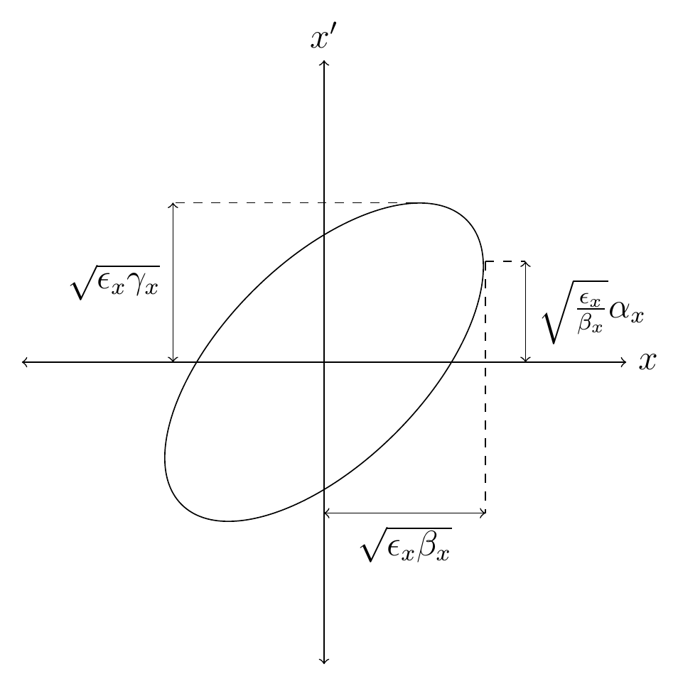
Figure 3: Phase space ellipse in the transverse x, x′ plane.
6.4 Beam Optics Parameterization#
The one-turn map M leads to stable motion whenever its eigenvalues \(\lambda^\pm_{I,II,III}=\exp(\pm i2\pi Q_{I,II,III})\) are complex and conjugate and the tunes \(Q_{I,II,III}\) are real. The one-turn map can be decomposed as
\[ \mathbf{M}= TRT^{-1}, \]where R is
\[ R=\left( \begin{array}{cccccc} \cos(2\pi Q_{I}) & \sin(2\pi Q_{I}) & 0 & 0 & 0 & 0\\ -\sin(2\pi Q_{I}) & \cos(2\pi Q_{I}) & 0 & 0 & 0 & 0\\ 0 & 0 & \cos(2\pi Q_{II}) & \sin(2\pi Q_{II}) & 0 & 0\\ 0 & 0 & -\sin(2\pi Q_{II}) & \cos(2\pi Q_{II}) & 0 & 0\\ 0 & 0 & 0 & 0 & \cos(2\pi Q_{III}) & \sin(2\pi Q_{III})\\ 0 & 0 & 0 & 0 & -\sin(2\pi Q_{III}) & \cos(2\pi Q_{III}) \end{array} \right) \]the rotation matrix, and
\[ T=\left( \begin{array}{cccccc} x_1 & x'_1 & y_1 & y'_1 & \sigma_1 & \delta_1\\ x_2 & x'_2 & y_2 & y'_2 & \sigma_2 & \delta_2\\ x_3 & x'_3 & y_3 & y'_3 & \sigma_3 & \delta_3\\ x_4 & x'_4 & y_4 & y'_4 & \sigma_4 & \delta_4\\ x_5 & x'_5 & y_5 & y'_5 & \sigma_5 & \delta_5\\ x_6 & x'_6 & y_6 & y'_6 & \sigma_6 & \delta_6 \end{array} \right) \]has the eigenvectors \(\vec{z}_i=(x_i,x'_i,y_i,y'_i,\sigma_i,\delta_i)\) for \(i=1,\ldots,6\) as rows, normalized so that \(TST^T=S\) (the same symplectic matrix from Section 6.1).
The optical properties of a lattice are conveniently described by a set of lattice functions. For a general six-dimensional case including coupling, three distinct oscillation modes — I, II and III — give rise to three sets of lattice functions7. Matrix T can be used to extract the coupled lattice functions by the following steps.
A point in the six-dimensional phase-space \(\vec{z}=(x,x',y,y',\sigma,\delta)\) can be described by six independent vectors \(\vec{z}_i=(x_i,x'_i,y_i,y'_i,\sigma_i,\delta_i)\) for \(i=1,\ldots,6\):
\[ \begin{aligned} x_1 &= \sqrt{\beta_{xI}(s)}\cos\Phi_{xI}(s) & x_2 &= \sqrt{\beta_{xI}(s)}\sin\Phi_{xI}(s) \\ x'_1 &= \sqrt{\gamma_{xI}(s)}\cos\tilde{\Phi}_{xI}(s) & x'_2 &= \sqrt{\gamma_{xI}(s)}\sin\tilde{\Phi}_{xI}(s) \\ x_3 &= \sqrt{\beta_{xII}(s)}\cos\Phi_{xII}(s) & x_4 &= \sqrt{\beta_{xII}(s)}\sin\Phi_{xII}(s) \\ x'_3 &= \sqrt{\gamma_{xII}(s)}\cos\tilde{\Phi}_{xII}(s) & x'_4 &= \sqrt{\gamma_{xII}(s)}\sin\tilde{\Phi}_{xII}(s) \\ x_5 &= \sqrt{\beta_{xIII}(s)}\cos\Phi_{xIII}(s) & x_6 &= \sqrt{\beta_{xIII}(s)}\sin\Phi_{xIII}(s) \\ x'_5 &= \sqrt{\gamma_{xIII}(s)}\cos\tilde{\Phi}_{xIII}(s) & x'_6 &= \sqrt{\gamma_{xIII}(s)}\sin\tilde{\Phi}_{xIII}(s) \end{aligned} \]and similarly for the \(y_i\), \(y'_i\), \(\sigma_i\) and \(\delta_i\) coordinates, using the lattice functions for the vertical and longitudinal planes, with \(\tilde{\Phi}_{yI}= \Phi_{yI} - \arctan(1/\alpha_{yI})\). Any point in the six-dimensional phase-space can then be written as
\[ \vec{z} = \left( \begin{array}{l} \sqrt{\epsilon_I}\sqrt{\beta_{xI}}\cos(\Phi_{xI}+\phi_I) + \sqrt{\epsilon_{II}}\sqrt{\beta_{xII}}\cos(\Phi_{xII}+\phi_{II}) + \sqrt{\epsilon_{III}}\sqrt{\beta_{xIII}}\cos(\Phi_{xIII}+\phi_{III}) \\ \sqrt{\epsilon_I}\sqrt{\gamma_{xI}}\cos(\tilde{\Phi}_{xI}+\phi_I) + \sqrt{\epsilon_{II}}\sqrt{\gamma_{xII}}\cos(\tilde{\Phi}_{xII}+\phi_{II}) + \sqrt{\epsilon_{III}}\sqrt{\gamma_{xIII}}\cos(\tilde{\Phi}_{xIII}+\phi_{III}) \\ \sqrt{\epsilon_I}\sqrt{\beta_{yI}}\cos(\Phi_{yI}+\phi_I) + \sqrt{\epsilon_{II}}\sqrt{\beta_{yII}}\cos(\Phi_{yII}+\phi_{II}) + \sqrt{\epsilon_{III}}\sqrt{\beta_{yIII}}\cos(\Phi_{yIII}+\phi_{III}) \\ \sqrt{\epsilon_I}\sqrt{\gamma_{yI}}\cos(\tilde{\Phi}_{yI}+\phi_I) + \sqrt{\epsilon_{II}}\sqrt{\gamma_{yII}}\cos(\tilde{\Phi}_{yII}+\phi_{II}) + \sqrt{\epsilon_{III}}\sqrt{\gamma_{yIII}}\cos(\tilde{\Phi}_{yIII}+\phi_{III}) \\ \sqrt{\epsilon_I}\sqrt{\beta_{\sigma I}}\cos(\Phi_{\sigma I}+\phi_I) + \sqrt{\epsilon_{II}}\sqrt{\beta_{\sigma II}}\cos(\Phi_{\sigma II}+\phi_{II}) + \sqrt{\epsilon_{III}}\sqrt{\beta_{\sigma III}}\cos(\Phi_{\sigma III}+\phi_{III}) \\ \sqrt{\epsilon_I}\sqrt{\beta_{\delta I}}\cos(\Phi_{\delta I}+\phi_I) + \sqrt{\epsilon_{II}}\sqrt{\beta_{\delta II}}\cos(\Phi_{\delta II}+\phi_{II}) + \sqrt{\epsilon_{III}}\sqrt{\beta_{\delta III}}\cos(\Phi_{\delta III}+\phi_{III}) \end{array} \right), \]where \(\phi_I\), \(\phi_{II}\) and \(\phi_{III}\) are the initial phases for modes I, II and III, and \(\sqrt{\epsilon_I}\), \(\sqrt{\epsilon_{II}}\), \(\sqrt{\epsilon_{III}}\) are their amplitudes. Under this definition, the effect of the one-turn map can also be expressed as
\[ \begin{aligned} \vec{z} &= \sqrt{\epsilon_I}\left(\vec{z}_1\cos(\phi_I+2\pi Q_I)+\vec{z}_2\sin(\phi_I+2\pi Q_I)\right)\\ &+ \sqrt{\epsilon_{II}}\left(\vec{z}_3\cos(\phi_{II}+2\pi Q_{II})+\vec{z}_4\sin(\phi_{II}+2\pi Q_{II})\right)\\ &+ \sqrt{\epsilon_{III}}\left(\vec{z}_5\cos(\phi_{III}+2\pi Q_{III})+\vec{z}_6\sin(\phi_{III}+2\pi Q_{III})\right) \end{aligned} \]The relation between the T matrix and the lattice functions can be found by
\[ \left( \begin{array}{cccc} \beta_{xI}=x_1^2+x_2^2 & \gamma_{xI}=x_1'^2+x_2'^2 & \alpha_{xI}=-(x_1x_1'+x_2x_2') & \Phi_{xI}=\arctan(x_2/x_1) \\ \beta_{xII}=x_3^2+x_4^2 & \gamma_{xII}=x_3'^2+x_4'^2 & \alpha_{xII}=-(x_3x_3'+x_4x_4') & \Phi_{xII}=\arctan(x_4/x_3) \\ \beta_{xIII}=x_5^2+x_6^2 & \gamma_{xIII}=x_5'^2+x_6'^2 & \alpha_{xIII}=-(x_5x_5'+x_6x_6') & \Phi_{xIII}=\arctan(x_6/x_5) \\ \beta_{yI}=y_1^2+y_2^2 & \gamma_{yI}=y_1'^2+y_2'^2 & \alpha_{yI}=-(y_1y_1'+y_2y_2') & \Phi_{yI}=\arctan(y_2/y_1) \\ \beta_{yII}=y_3^2+y_4^2 & \gamma_{yII}=y_3'^2+y_4'^2 & \alpha_{yII}=-(y_3y_3'+y_4y_4') & \Phi_{yII}=\arctan(y_4/y_3) \\ \beta_{yIII}=y_5^2+y_6^2 & \gamma_{yIII}=y_5'^2+y_6'^2 & \alpha_{yIII}=-(y_5y_5'+y_6y_6') & \Phi_{yIII}=\arctan(y_6/y_5) \\ \beta_{\sigma I}=\sigma_1^2+\sigma_2^2 & \gamma_{\sigma I}=\delta_1^2+\delta_2^2 & \alpha_{\sigma I}=-(\sigma_1\delta_1+\sigma_2\delta_2) & \Phi_{\sigma I}=\arctan(\sigma_2/\sigma_1) \\ \beta_{\sigma II}=\sigma_3^2+\sigma_4^2 & \gamma_{\sigma II}=\delta_3^2+\delta_4^2 & \alpha_{\sigma II}=-(\sigma_3\delta_3+\sigma_4\delta_4) & \Phi_{\sigma II}=\arctan(\sigma_4/\sigma_3) \\ \beta_{\sigma III}=\sigma_5^2+\sigma_6^2 & \gamma_{\sigma III}=\delta_5^2+\delta_6^2 & \alpha_{\sigma III}=-(\sigma_5\delta_5+\sigma_6\delta_6) & \Phi_{\sigma III}=\arctan(\sigma_6/\sigma_5) \end{array} \right), \]where \(a_i=\frac{\partial a}{\partial z_i}\), that is, \(x_1=\frac{\partial x}{\partial x}, x_2=\frac{\partial x}{\partial x'}, x_3=\frac{\partial x}{\partial y}, \ldots\)
To obtain the lattice functions at another point of the ring, it's enough to transport the generating eigenvectors through the lattice and read the relations above again at the new location.
6.5 Non-Linear motion#
If the motion is linear and the one-turn map has stable eigenvalues, the motion of a single particle is bounded for an infinitely large number of turns, and any phase-space point can be associated with a linear invariant. However, the motion is perturbed whenever a non-linear force is present, leading to chaotic motion, with particle trajectories that are no longer bounded inside an ellipse of the phase-space.
In the case of weak non-linearities, the motion is still stable for a long time within a relatively large area of phase-space, whose projection onto the x, y plane is usually comparable to the vacuum pipe's cross-section. If that region were too small, not many particles could circulate in the machine before being lost — but it is typically not very large either, since non-linear elements are deliberately added to compensate for energy errors and to spread the frequency of the natural modes.
For weak non-linearities, it still makes sense to calculate linear invariants such as amplitudes, tunes and lattice functions, which this time will evolve turn by turn. It is also useful to track particles with very close-by initial coordinates, to study the sensitivity of the motion to small variations of the initial conditions. Instead of looking directly at the trajectory's coordinates, the coefficients of the linear parameterization (such as ε and φ) offer a more stable and decoupled set of coordinates, whose only source of variation comes from the non-linear motion — since, under ideal linear motion, they would otherwise be invariant.
SixTrack computes both particle trajectories and linear lattice functions, and it's the combined analysis of the two that forms the foundation of its post-processing routines.
The next article in this series walks through SixTrack itself and the Fortran post-processing subroutines built on top of these foundations, and the one after that covers porting that post-processing to Python and SQL.
-
Schmidt, F. (1990). Sixtrack. CM-P00049314. ↩︎
-
McIntosh, E., & De Maria, R. (2012). The SixDesk run environment for SixTrack. CERN-ATS-Note-2012-089 TECH. ↩︎
-
Giovanozzi, M., Zacharov, I., & Rivkin, L. (2012). LHC@Home: A Volunteer computing system for Massive Numerical Simulations of Beam Dynamics and High Energy Physics Events. IPAC2012 Proceedings, EPFL-CONF-181616. ↩︎
-
Anderson, D. P. (2004). BOINC: A system for public-resource computing and storage. Grid Computing, 2004. Proceedings. Fifth IEEE/ACM International Workshop on, 4-10. ↩︎
-
De Maria, R., & Fjellstrom, M. (2013). Sixtrack physics manual (draft). ↩︎
-
Jackson, J. D. (1962). Classical electrodynamics (Vol. 3). Wiley. ↩︎
-
Ripken, G., & Willeke, F. (1988). Methods of Beam Optics. DESY. ↩︎