Vectorizing and parallelizing ROOT's fits
This article is part of a series that I'm slowly publishing, and it still has several broken links referencing unpublished articles.
Fitting of data distributions is one of the most demanding and computing-intensive activities when performing data analysis on the results of the LHC.
In order to take full advantage of new computer architectures, and to maintain or even improve performance with increasing amounts of data to analyze, parallelization and vectorization have been introduced in the ROOT mathematical and statistical libraries.
The tools for parallelism described in ROOT's executors and SIMD in ROOT can be applied together when parallelizing the minimization process for solving fitting problems. As a result of the substantial work done on developing and integrating these parallelization tools in ROOT, vectorization and parallelization have been introduced in ROOT's fitting interfaces, requiring minimal changes in user code. To improve the speed up, ROOT's main fitting methods, introduced in Section 6.1, have been parallelized both at data-level (Section 6.3) and task-level (Section 6.4).
We report on the improvements obtained by adding support for SIMD vectorization and multithreaded parallelization in the function evaluation with a typical example from HEP data analysis. In Section 6.5, we show how the different evaluations of the likelihood and the least square functions used for fitting ROOT histograms and datasets represented by ROOT trees perform for this case.
6.1 Fitting fundamentals#
Fitting is one of the most recurrent and fundamental operations in HEP, as it provides valuable information about the distribution of the observed data. In this section we introduce the foundations of likelihood fitting, introducing the concepts of likelihood and likelihood function, and focusing on two methods to estimate the parameters that maximize the likelihood function: maximum likelihood and least squares.
The likelihood function#
Consider the hypothesis H as a conjecture over the probability P(x|H) of the observed data x. If P(x|H) were to define the probability density function (p.d.f.) for the data as a function of H, we would then call L(H) = P(x|H) the likelihood of H.
If the hypothesis is characterized by the typically unknown parameters θ, then L(θ) = P(x|θ) is called the likelihood function.
The likelihood function plays a central role in the fitting process, which ultimately consists of inferring θ from x so that we find the probability mass or density function (in this case L(θ)) that better adjusts to the observed data. For this purpose, we need good estimators of the parameters.
For instance, we are frequently in need of good estimators for the median, mean and variance parameters of a distribution. In this case, a good choice of estimators is to set the median to the sample median and to estimate the mean μ̂ and the variance σ̂² with the unbiased estimators given by the equations
\[ \hat{\mu} = \frac{1}{n}\sum_{i=1}^n x_i, \qquad \hat{\sigma}^2 = \frac{1}{n-1}\sum_{i=1}^n (x_i - \hat{\mu})^2 \]Maximum Likelihood#
Given a set of parameters θ, we want to obtain the set of estimators θ̂ that maximize the likelihood function. In other words, the maximum likelihood estimate follows
\[ \hat{\theta} = \max L(\theta), \qquad \forall \theta \in \Theta,\ \hat\theta \in \hat\Theta \]However, it is frequently more convenient to work with the natural logarithm of the likelihood function, \(\ln L\), finding the estimators by solving the equation
\[ \frac{\partial \ln L}{\partial \theta_i} = 0, \qquad i = 1,\ldots,N. \]The likelihood function formulation depends on the nature of the data. For example, if the data consists of a fixed number n of independent and identically distributed values following the same p.d.f., the likelihood becomes
\[ L(\theta) = \prod_{i=1}^n f(x_i;\theta) \]where f(x, θ) is the p.d.f. of observing the data x given the set of parameters θ. If the data does not consist of a fixed number of events, but the probability to observe n events follows a Poisson distribution with mean μ depending on the parameter θ, then we obtain the extended likelihood function formula:
\[ L(\theta) = \frac{\mu^{n}}{n!}e^{-\mu}\prod_{i=1}^n f(x_i;\theta) \]Binned maximum likelihood#
If the data sample contains a large number of values, it is usually convenient to represent it as a histogram, classifying the values in N bins.
If, again, the n bins created out of ntot events are independent and follow a Poisson distribution, the likelihood function takes the form
\[ f_P(n;\theta) = \frac{\mu_i^{n}}{n_i!}e^{-\mu_i}\prod_{i=1}^n f(x_i;\theta), \]where μᵢ are the mean values of the bins described as functions of θ, and μtot = Σᵢ μᵢ is the mean of the ntot original events of the Poisson distribution.
By using the likelihood ratio λ(θ) = fP(n; θ)/f(n; μ̂), we can obtain, in addition, an indicator of the “goodness of fit”1:
\[ -2\ln\lambda(\theta) = 2\sum_{i=1}^N \left[ \mu_i(\theta) - n_{i}+n_i \ln \frac{n_i}{\mu_i^{n}} \right] \]Least squares#
Besides the maximum likelihood, there is an alternative way of inferring the parameters by using the method of the least squares2.
Given a set of N independent measurements at point yᵢ, with mean μ(xᵢ; θ) and variance σᵢ², the least squares estimators Θ̂ for the unknown parameters Θ can be defined by the equation:
\[ \chi^2(\theta) = \sum_{i=1}^N\frac{(y_i-\mu(x_i;\theta))^2}{\sigma_i^2}, \qquad \forall \theta \in \Theta \]where the parameters minimizing χ²(θ) maximize the likelihood L. If yᵢ were to be Gaussian distributed, the least squares method would be equivalent to that of the maximum likelihood described above.
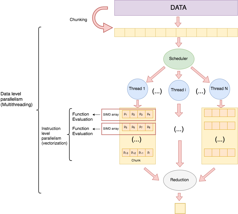
Figure 6.1: Depiction of the parallelization of the fitting. The parallelization at task-level involves chunking, multithreaded mapping (distribution and evaluation) and reduction to a single result. At data-level, we vectorize the model function evaluation.
6.2 Parallelization of the fitting in ROOT#
In this section, we study the parallelization of the maximum likelihood, the binned likelihood and the least squares methods described above.
Figure 6.1 illustrates the parallelization process followed in each one of the algorithms and the way each layer of parallelism is exploited in a multicore computer.
We start by dividing the data into N chunks and distributing them to N tasks that will run in M threads (Chunking stage). The Map stage of the MapReduce implementation of choice — TProcessExecutor (see TProcessExecutor) for multiprocessing, TThreadExecutor (see TThreadExecutor) for multithreading — is responsible for the distribution of the tasks to the threads (Distribution stage).
Although the clustering of the data can be delegated to the user, we can take advantage of the chunking capabilities of the MapReduce executors as well. However, since in this case the nature of the data and the evaluation functions are opaque to the fitting interfaces, it is difficult to infer the most efficient number of chunks without any input from the user.
Notwithstanding, we provide a heuristic function to infer an appropriate number of chunks, depending on the size of the datum and within a range given by empirical experimentation (see Section 6.4). This number of chunks should be large enough to improve balancing, but within a certain limit to avoid that the overhead of task creation undermines the balancing benefits.
Every task of the Map stage evaluates the function on C events, where C = nEvents / N is the chunk size (Evaluation stage). If the user provides a vectorized function that takes ROOT's SIMD types as parameters, while still evaluating C events, the number of function evaluations per task is reduced from C to roughly C/S. Here, S is the number of double types fitting into the SIMD array size of the instruction set, as the ROOT fitting interfaces are designed to only evaluate on double. That is to say that the least squares equation becomes a double sum over chunks and over the SIMD arrays within each chunk, where j iterates over the number of chunks, i iterates over the number of SIMD arrays of size S that fit in a chunk, and the SIMD array xij is the i-th SIMD array in the j-th chunk or partition of the data point x.
Once all the data points have been evaluated, the Reduce stage will be invoked on the returned map vector (Reduction stage). Note that providing a vectorized function will also reduce the size of the returned Map std::vector, which will diminish the cost of the Reduce phase.
All this is possible thanks to the parallelization of the fitting functions and the “templatization” of ROOT's fitting interfaces.
The fitter, the interface between the minimizer and the fitting interfaces, uses the data and the model function to implement the objective function (χ², Max. Likelihood), whose implementation is parallelized at task-level by TThreadExecutor and TProcessExecutor (Section 6.4). The fitter also provides the objective function to the minimizer, which can compute internally the gradient using numerical differentiation, or it can be passed by the fitter using the gradient of the model function.
The fitter requires the model function received to be described by a generic interface that accommodates the function evaluation in ROOT, which can be used for fitting and other numerical algorithms. For their convenience, we require the users to pass the model function to the fitter via the TF1 class. The TF1 instance is then wrapped in the generic interface, which has been extended for vectorization using templates. ROOT also provides a similar interface for gradient evaluation.
In some cases, we may want to compute externally the numerical derivatives of the model function (e.g. to save computational time). This external derivation is provided by the user by leveraging ROOT's gradient interfaces. The user's derivative function is then propagated to the gradient function of the minimizer of choice via the fitter, and evaluated sequentially or in parallel either at data-level or task-level. The implementations that use these gradient interfaces have also been parallelized and vectorized.
In the following sections we explore in more detail the challenges confronted, technical details and the implementation decisions during the exploitation of data-level parallelism and task-level parallelism of the fitting in ROOT.
6.3 Vectorization#
ROOT provides two data classes for the representation of the fitting data: binned and unbinned. These classes are filled with the ROOT user data object, such as histograms or trees, and provide the necessary interfaces for the fitter to manipulate the data.
Both the binned and unbinned data classes have been adapted to exploit data-level parallelism. This type of parallelism is implemented in the fitting using VecCore3 (see VecCore), to adapt the fitting interfaces to vectorize the operations in the evaluation of the model function provided by the user.
For this, we need to modify the way ROOT stores the fitting data in the data structures mentioned above and to provide padding mechanisms for safe lecture and storage of the data in the SIMD types used by the vectorized fitter. Furthermore, we need to template the fitting interfaces and to vectorize the implementation of the objective function to read and operate on SIMD arrays.
From Array of Structures to Structure of Arrays#
Efficient vectorization requires changes in the way ROOT stores data coordinates. Prior to these changes, ROOT stored these data in an object-oriented way; that is, for each data point, all its coordinates were stored consecutively, in arrays of structures (AOS). For example, for a three-dimensional data point, ROOT stored the three coordinates x, y, z contiguously in memory, that is, the data array was stored as (x, y, z)n = (x0, y0, z0, …, xn, yn, zn).
When loading memory into a SIMD array, we provide the start address of the data and we gather as much contiguous data as the size of the SIMD array indicates. This means that, for correct loading of the coordinates in SIMD arrays, the points' coordinates should be stored in contiguous positions in memory; otherwise the memory loaded into the SIMD array might be incorrect or corrupted. As we want to evaluate several points per coordinate at a time, we need to store the N coordinates in N aligned vectors of data points, or structures of arrays (SOA), that is (x, y, z)n = (x0, …, xn, y0, …, yn, z0, …, zn).
Padding#
SIMD instruction sets distinguish between two kinds of instructions: packed and scalar.
A scalar instruction is evaluated on one data element at a time while a packed instruction is evaluated over a full SIMD array. Note that these are the only two options available: if the datum size is not a multiple of the SIMD array size for a certain type, the last (incomplete) array will either be loaded as a set of scalars or require padding to load it as a packed SIMD array.
We have developed a padding mechanism in order to avoid loading wrong memory addresses into SIMD arrays, i.e. filling the empty positions of the SIMD array with the last data element if the remaining data to load is less than the SIMD vector size. The choice of filling with the last data element is not arbitrary: it is a requisite for the padding to be composed of values that guarantee safe evaluations. This avoids invalid operations (e.g. dividing by zero when padding with the default value for the type) and guarantees that the operation to be performed will be correct. This padding mechanism has been implemented for the coordinates, and for the values and the error in the case of binned data representations.
Vectorization of ROOT Math interfaces#
ROOT Math interfaces to functions and numerical algorithms have been designed to accept only double precision types. Instead of adding extra overloads to be able to operate with SIMD arrays, we decided to template all fitting and function interfaces, retaining the existing classes as an alias of the new templated ones instantiated on double. The structure of the function interfaces in ROOT prior to their templatization gives a sense of the complexity of this task: a dense web of inheritance between the fitting classes, the minimizer classes, and the gradient and parametric function interfaces, which all needed to carry a SIMD type parameter through every layer without breaking existing user code.
VecCore is the SIMD library of choice to express vectorization in ROOT, for the reasons explained in SIMD in ROOT. We leverage VecCore types to specify the new type ROOT::Double_v that allows us to work with SIMD types inside ROOT and expose them for user-specified functions.
Once we obtain the user function, we provide full compatibility with most of the old scripts. This means that, in order to benefit from a vectorized evaluation of the fitting, users will only need to vectorize their function, which in some cases may only require changing the data and return type. The user can also easily create vectorized functions by using TMath methods or TFormula (see Putting ROOT's parallel tools to the test) instances.
In order to achieve this backward compatibility, and as a fundamental class of the fitting process, we also developed templated overloads of the TF1 function type constructors, and implemented the necessary internal mechanisms for evaluation on SIMD types, as discussed in Generating Julia fractals with TF1.
6.4 Multiprocessing and multithreading#
Our task-level parallelization of the fitting process targets the loop over the data elements in each one of the fitting functions. This approach requires making all the invoked functions within the loop body scope thread-safe, removing all dependencies on previous iterations, and adapting the code to the interface provided by TExecutor.
As a requirement from TThreadExecutor and TProcessExecutor's interface, the body of the loop evaluation on the datum has been transformed into a callable that evaluates the data on a single point (or SIMD array size points when applying vectorization) and returns the evaluation result. This callable plays the role of the mapping function. The reduction function, another callable, will be adapted to each fitting model, as well as the returned types, from the mapping function. An example of this process is provided in Listing 6.1.
//Halves accumulation loop
unsigned sum;
for(unsigned i=0; i<N; i++){
    sum+=i/2;
}

// Same loop parallelized with TThreadExecutor
auto singleEvaluation = [](const unsigned &i) {
    return i/2;
}
auto reduceFunction = [](const std::vector<unsigned> &v) {
    return std::accumulate(v.begin(), v.end(), 0U);
}

ROOT::TThreadExecutor pool;
pool.MapReduce(singleEvaluation, ROOT::TSeq<unsigned>(N), reduceFunction);
Listing 6.1: Porting a traditional loop to TThreadExecutor. We implement in one callable (singleEvaluation) the operation to perform on a single point, and in another one (reduceFunction), the function to reduce the multiple partial results. Finally, we create an instance of TThreadExecutor and call its MapReduce function, which will receive as parameters both callables and, in this case, a sequence of unsigned integers.
For performance, we also propose a heuristic chunking function (Listing 6.2) based on empiric experience and the size of the data that, additionally, limits the potential number of tasks within a fixed interval. The objective is to generate a number of chunks which facilitates attaining work balancing to the TBB scheduler, but which is not so small as to be influenced by the TBB tasks creation overhead. We could improve this function by timing both the evaluation of a single data element and the overhead of creating a task in TBB. This proposal would make sense with data of large size, as the time to evaluate a single additional data point is negligible.
unsigned setAutomaticChunking(unsigned nEvents){
      auto ncpu  = std::thread::hardware_concurrency();
      if (nEvents/ncpu < 1000) return ncpu;
      return nEvents/1000;
      //return ((nEvents/ncpu + 1) % 1000) *40 ; //arbitrary formula
}
Listing 6.2: Heuristic function to set an appropriate number of tasks, dependent on the size of the datum (nEvents) and limiting the maximum number of tasks to process.
We also defined the new type ROOT::Fit::ExecutionPolicy, representing the different execution policies, with the options described in Listing 6.3.
In order to specify the execution policy when calling the fit from a histogram, we extended its interfaces with the options "SERIAL", "MULTITHREAD" — not necessary if ImplicitMT is enabled — and "MULTIPROCESS".
namespace ROOT{
   namespace Fit{
      enum class ExecutionPolicy {
         kSerial,
         kMultithread,
         kMultiprocess
      };
   }
}
Listing 6.3: Execution policies available for fitting, representing the serial case, the multithreaded case and the multiprocessed case.
As with the rest of ROOT's parallel tools, both implicit and explicit multithreading are offered for the fit: setting the execution policy explicitly gives users and framework developers fine control when it is needed, while leaving it on "SERIAL" and enabling implicit multithreading globally lets the same code benefit from parallelism transparently, for user convenience, flexibility and interface coherency.
6.5 Case example: A typical fit#
As an example of how the changes introduced in ROOT can contribute to accelerate the fitting, we choose a fit of the diphoton invariant mass distribution resulting from a Higgs boson (Figure 6.3). Listings 6.4 and 6.5 offer a comparison of the scalar code for this benchmark fit against the code needed for a fully parallelized (multithreading plus vectorization) implementation of the same fit.
//Example Fit: Implementation of the scalar function
double func(const double *data, const double *params)
{
   return params[0] * exp(-(*data + (-130.)) * (*data + (-130.)) / 2) +
          params[1] * exp(-(params[2] * (*data * (0.01)) - params[3] *
          ((*data) * (0.01)) * ((*data) * (0.01))));
}

auto f = TF1("fScalar", func, 100, 200, 4);
f.SetParameters(1, 1000, 7.5, 1.5);
TH1D h1f("h1f", "Test random numbers", 12800, 100, 200);
h1f.FillRandom("fScalar", 1000000);
h1f.Fit(&f);
Listing 6.4: Traditional scalar implementation.
//Example Fit: Implementation of the vectorized function
ROOT::Double_v func(const ROOT::Double_v *data, const double *params)
{
   return params[0] * exp(-(*data + (-130.)) * (*data + (-130.)) / 2) +
          params[1] * exp(-(params[2] * (*data * (0.01)) - params[3] *
          ((*data) * (0.01)) * ((*data) * (0.01))));
}

// Enable implicit parallelization
ROOT::EnableImplicitMT();

//This code is totally backwards compatible
auto f = TF1("fvCore", func, 100, 200, 4);
f.SetParameters(1, 1000, 7.5, 1.5);
TH1D h1f("h1f", "Test random numbers", 12800, 100, 200);
h1f.FillRandom("fvCore", 1000000);
h1f.Fit(&f);
Listing 6.5: Vectorized plus parallelized implementation.
In Listing 6.5 we provide the parallelization and vectorization while maintaining the previous programming model. This is an important achievement, as users can now benefit from multiple levels of parallelization without modifying their old scripts. Starting from line 9 in Listing 6.4, and line 13 in Listing 6.5, the code related to the fitting operations is exactly the same. The only changes required for fitting the data in the vectorized and parallelized case — Listing 6.5 — are additions on top of the current workflow.
First, in order to profit from the implicit task parallelization, the user only needs to call EnableImplicitMT (line 10 of Listing 6.5). This will activate all the mechanisms in ROOT that provide thread safety and parallelize all the operations that allow implicit multithreading in ROOT, such as the fitting. For vectorization, the user needs to provide a vectorized function, which in this case only implies changing the data parameter type and the return type — to the new ROOT::Double_v type, representing a SIMD array of double — as shown in line 2 of Listing 6.5.
We perform three different types of fits, χ² and Poisson likelihood in the binned case and Maximum Likelihood in the unbinned case, to the invariant mass distribution, studying the speed up in each one of these cases.
In all experiments, the final sum of the partial results (the Reduction stage in Figure 6.1) is computed sequentially and in the same order for the sake of numerical reproducibility. We measured the fitting times normalized to the number of objective function calls made by the fitter, as the nature of the minimization problems makes the number of calls fluctuate between examples, due to numerical precision, and influence the measured times.
Individual evaluations of the objective function#
We first measure the time taken by a single evaluation of each objective function, compiled with gcc 6.2 on a 4-core Broadwell desktop server with 8 GB of RAM, over 120001 bins in the binned case and 120001 points in the unbinned case. We observe close to ideal results both when exploiting task-level parallelism (Parallelized) and data-level parallelism (Vectorized). The best results are obtained with the combination of the two levels of parallelism, with a remarkable speed up even in the χ² evaluation, though the speed up there is lower than for the other two models.
| Objective function / Model | Time (µs) | Speed up |
|---|---|---|
| χ² / Sequential | 752.14 | 1 |
| χ² / Vectorized | 232.60 | 3.23 |
| χ² / Parallelized | 214.82 | 3.50 |
| χ² / Vectorized + Parallelized | 80.34 | 9.36 |
| Poisson Likelihood / Sequential | 1283.20 | 1 |
| Poisson Likelihood / Vectorized | 240.83 | 5.33 |
| Poisson Likelihood / Parallelized | 409.62 | 3.13 |
| Poisson Likelihood / Vectorized + Parallelized | 89.58 | 14.33 |
| Unbinned Likelihood / Sequential | 1188.25 | 1 |
| Unbinned Likelihood / Vectorized | 361.99 | 3.28 |
| Unbinned Likelihood / Parallelized | 367.04 | 3.24 |
| Unbinned Likelihood / Vectorized + Parallelized | 89.85 | 13.22 |
Table 6.1: Measured times and speed up for individual calls of the objective functions (4-core Broadwell, 8 GB RAM, AVX2). Measured by the microbenchmarking library Google Benchmark4, averaging thousands of calls. Evaluated over 120001 bins in the binned case and 120001 points in the unbinned case.
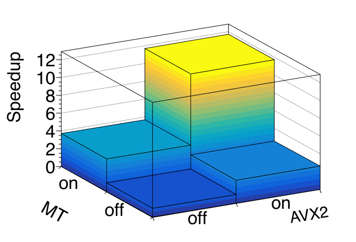
Combined speed up from switching multithreading (MT) and AVX2 vectorization on and off independently, for the Poisson likelihood objective function. Each level of parallelism contributes on its own, and the two compound when applied together.
Notice the super-linear speed up when vectorizing the Poisson likelihood. This is due to improvements (e.g. fused multiplication and addition) in some vectorized operations such as the computation of the logarithm, which in this case is called several times per data point evaluation.
A complete fit#
For a more relevant use case, we benchmark a complete fit. A fit is a minimization process that consists in several calls to the objective function by a minimizer — external in ROOT's case — that will make educated guesses on the estimators until it reaches an optimal solution.
The interactions between the fitting model functions and the minimizer are handled through the fitter, the ROOT class that manages the fitting process. Because the calls to the fitter interface can add overhead in addition to the evaluation of the function, benchmarking a complete fit is important.
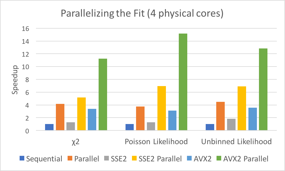
Figure 6.5: Performance of the fit (4-core Broadwell, 8 GB RAM) for the three objective functions, comparing the sequential, parallel, SSE2, SSE2 parallel, AVX2 and AVX2 parallel cases. Evaluated over 120k bins in the binned fits and 120k points in the unbinned fit.
Figure 6.5 and Table 6.2 report the speed up attained by the parallel fitting, compiled with gcc 6.2 on a desktop server equipped with a 4-core Haswell processor and 8 GB of RAM, and distinct sets of vectorization instructions and evaluation functions.
| Objective function / Model | Time (s) | Speed up |
|---|---|---|
| χ² / Sequential | 12.11 | 1 |
| χ² / Parallel | 3.20 | 4.19 |
| χ² / SSE | 8.54 | 1.29 |
| χ² / SSE2 parallel | 4.74 | 5.18 |
| χ² / AVX2 | 4.18 | 3.41 |
| χ² / AVX2 parallel | 1.60 | 11.23 |
| Poisson Likelihood / Sequential | 16.05 | 1 |
| Poisson Likelihood / Parallel | 4.24 | 3.74 |
| Poisson Likelihood / SSE | 15.25 | 1.3 |
| Poisson Likelihood / SSE2 parallel | 2.33 | 6.95 |
| Poisson Likelihood / AVX2 | 6.57 | 3.11 |
| Poisson Likelihood / AVX2 parallel | 1.40 | 15.18 |
| Unbinned Likelihood / Sequential | 3.09 | 1 |
| Unbinned Likelihood / Parallel | 0.82 | 4.48 |
| Unbinned Likelihood / SSE | 1.69 | 1.82 |
| Unbinned Likelihood / SSE2 parallel | 0.37 | 6.90 |
| Unbinned Likelihood / AVX2 | 0.86 | 3.59 |
| Unbinned Likelihood / AVX2 parallel | 0.23 | 12.86 |
Table 6.2: Times and speed up of the fit (4-core Broadwell, 8 GB RAM) for different pairs of objective function and execution policy. Evaluated over 120k bins in the binned fits and 120k points in the unbinned fit. Complements Figure 6.5.
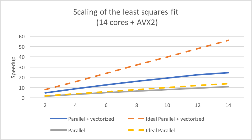
Figure 6.6: Scaling of the least squares fit with an increasing number of cores (14-core Xeon, AVX2, 64 GB RAM).
In Figure 6.6 and Table 6.3, we show the scaling of multithreaded operations on a 14-core Xeon processor with AVX2 and 64 GB of RAM. While it scales in the multithreaded scalar case, suboptimal vectorization limits the total speed up.
| Cores | 2 | 4 | 6 | 8 | 10 | 12 | 14 |
|---|---|---|---|---|---|---|---|
| Parallel | 1.78 | 3.43 | 5.18 | 6.59 | 8.21 | 9.54 | 10.9 |
| Ideal Parallel | 2 | 4 | 6 | 8 | 10 | 12 | 14 |
| Parallel + vectorized | 4.80 | 8.99 | 12.66 | 16.08 | 19.24 | 22.51 | 24.57 |
| Ideal Parallel + vectorized | 8 | 16 | 24 | 32 | 40 | 48 | 56 |
Table 6.3: Execution time recorded in seconds for a complete fit (Haswell, 14 cores, 8 GB RAM) with an increasing number of cores. Complements Figure 6.6.
It is also interesting to show how different compilers behave when vectorizing the evaluation of the model function. We assess the impact of distinct compiler technology next.
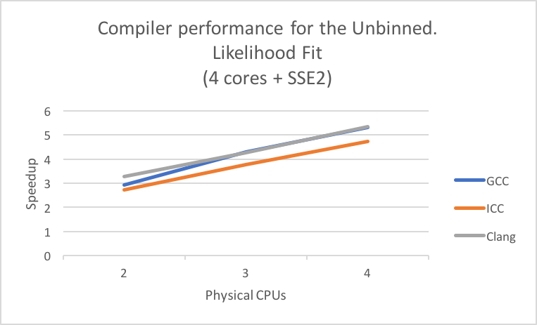
Figure 6.7: Compiler comparison (gcc 6.2, clang 3.8, icc 17) for the execution time of the maximum likelihood evaluation, sequentially and vectorized with SSE2. Carried out in double precision.
Observing Figure 6.7, we find out that icc 17 performs a more aggressive auto-vectorization than the other compilers, matching the explicitly vectorized times. For a fairer comparison, avoiding autovectorization when compiling, the results between compilers are similar, with icc slightly outperformed by clang and gcc, and all three compilers continue to track each other closely as the number of threads increases.
6.6 Conclusions#
In this chapter we demonstrate that, with the appropriate tools, we can exploit parallelism at several levels when fitting models in ROOT and, at the same time, preserve the user interfaces. We have shown how, as a result, the users can now vectorize and parallelize their original code and profit from a significant speedup.
We described the necessary changes to improve the performance of the vectorization introduced for SIMD in ROOT, from structuring our data in a Structure of Arrays to achieve data alignment, to providing safety mechanisms, such as that described for the padding. In addition, we applied the knowledge obtained from the task granularity analysis to define a heuristic that contributes to balancing the parallel workload. Finally, we parallelized the evaluation of the different objective functions by deploying the executors and adapting the processing of the event loop to a MapReduce model.
We utilized a real use case to benchmark the parallelization at task-level (multithreading) and data-level of the unbinned maximum likelihood, the Poisson likelihood and the least-square methods, on individual evaluations and on a complete fitting process for each of the objective functions.
Results differ between objective functions, but in all the benchmarked cases we obtained good acceleration factors when vectorizing, and remarkable ones when parallelizing at task-level. The combination of both task-level and data-level parallelism produces the best results, and both speed up and execution times are consistent across compilers.
-
Baker, S., & Cousins, R. D. (1984). Clarification of the use of chi-square and likelihood functions in fits to histograms. Nuclear Instruments and Methods in Physics Research, 221(2), 437-442. link ↩︎
-
Least squares: https://en.wikipedia.org/wiki/Least_squares ↩︎
-
Amadio, G., Canal, P., & Wenzel, S. (2017). root-project/VecCore: Release v0.4.2. link ↩︎
-
Google Benchmark: https://github.com/google/benchmark ↩︎