Putting ROOT's parallel tools to the test
This article is part of a series that I'm slowly publishing, and it still has several broken links referencing unpublished articles.
The parallel tools and libraries described throughout this series yield significant performance improvements for ROOT and align with its ongoing modernization effort. These tools have been extensively deployed throughout ROOT: training of Deep Neural Networks, parallel merging of files, parallel processing of ROOT trees, vectorizing the fit, vectorizing mathematical functions and user-defined formulas, parallel writing of histograms, parallel evaluation of the event loop in RDataFrame, and so on.
This article serves as a showcase for some of the performance improvements granted by the utilities for parallelism at task-level and data-level introduced in the previous articles of the series. Section 7.1 describes the improvements obtained when parallelizing ROOT's standalone tool for merging ROOT files, hadd, using the multiprocess executor of ROOT, TProcessExecutor. In Section 7.2, we introduce a code exploring a potential model of new Physics, and we benchmark the performance of its RDataFrame implementation against the original ad-hoc highly optimized version of the same code. Finally, Section 7.3 compares and reports on the performance of vectorizing mathematical functions at runtime via TFormula.
7.1 Merging of ROOT files#
Merging ROOT files is a common but expensive operation. ROOT offers a tool for this purpose, hadd, that could benefit from parallelization. Concretely, hadd is a standalone application distributed with ROOT whose objective is to merge several ROOT files containing ROOT trees or histograms into a new file, by exploiting the Merge() method of these classes and ROOT's file-managing utilities, e.g. TFileMerger1.
This is an easily parallelizable procedure, for instance, by relying on recursive hierarchical merging. The most obvious implementation is to perform the merge following a binary tree structure: each node of the tree constitutes a task that merges two files into one, and these tasks are computed concurrently. Parallelizing the merging of the ROOT files in this way would grant a potential speed up in the number of merges of
\[ S_u = \frac{n}{2^{\log_2 n - \log_2 m}-1} = \frac{mn}{n-m}, \]where the sequential tree for n = 2k+1 files has n − 1 nodes, or binary merge operations, and m = 2i is the number of parallel processing elements.
Nevertheless, real world problems are seldom this perfect. For instance, the number of files may not be a power of two, and then the shape of the tree does not correspond to that of a full binary tree. In addition, the number of processing units may not be a divisor of the number of files, and, in that case, it is better performance-wise to distribute the files such that the leaf operations do not constitute a binary merge.
Due to the particularities of the Merge() operation in ROOT, in which a collection of ROOT objects is merged into the first element of the collection, the full combination of the objects requires n − 1 merges for n files. With n files distributed among the m processing units, and each one of the leaves of the tree performing a sequential merge of the files it was assigned, the potential acceleration factor that we can obtain in the number of merges is:
However, while merging in a binary tree is theoretically the most efficient option, in practice, the overhead caused by the implementation of a partial binary file merging operation, and the limitations of the I/O subsystem (opening a file, creating a file merger, writing results on disk), make this option less practical. Instead, we adopt a two-step MapReduce2 solution where we distribute the files uniformly between the p workers, and then we perform partial reduction in each of the workers ("greedy" reduce), only to reduce these partial results one last time to obtain the final result.
The theoretical maximum speedup that we can obtain when merging files in two steps is governed by the equation
\[ S_u = \frac{n(n-1)}{\frac{n}{m}+m-2}, \]where n is the number of items to process and m is the number of processing workers.
We developed this last solution in a parallel MapReduce implementation of hadd, relying on the multiprocess executor of ROOT, TProcessExecutor3, for merging ROOT objects stored in ROOT files. Without changing the original user interface, the command remains as simple as:
# Merge 48 histogram files using a 4-worker TProcessExecutor-backed hadd
hadd -j 4 merged.root input_*.root
Listing 7.1: Invoking the parallel, MapReduce-based implementation of hadd with 4 worker processes.
Most frequently, a ROOT file contains data in either ROOT trees or ROOT histograms. We test the parallel merging of histogram files with a file from the official CMS data quality monitoring repository, a real case with around 12.5 MB of hundreds of histograms in a complex hierarchy of directories, which should result in a large workload. We merge in parallel the same file duplicated N times for balancing purposes, on an Intel Core i7-4790 desktop server with 4 physical cores (8 logical threads) at 3.6 GHz and 8 GB of RAM4, measured with the standard high resolution clock of C++ and each measurement averaged over several executions.
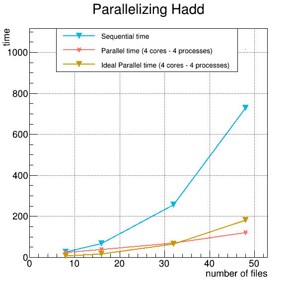
Figure 7.1: Time to merge an increasing number of histogram files: sequential execution, 4-core/4-process parallel execution, and the theoretical ideal parallel time.
Figure 7.1 shows that the time needed for the sequential merge grows rapidly with the number of files, while the parallel execution stays close to the ideal curve. By default, TProcessExecutor deploys as many workers as logical cores—in this case 8—which, as we observe next, does not positively affect performance.
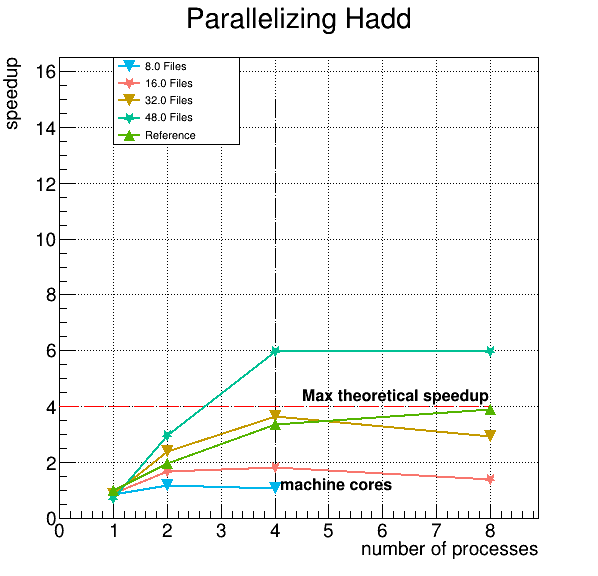
Figure 7.2: Speed up merging with hadd a different number of ROOT files containing histograms, with an increasing number of processes. The dashed horizontal line marks the theoretical maximum speed up for the available machine cores.
Figure 7.2 compares the speed up obtained for a varying number of files against the number of processes used and the reference maximum speed up for the available cores. We notice that, when the number of files increases, the speed up rapidly approaches and even exceeds the naive core-count reference, as larger workloads amortize the fixed cost of worker creation and file-opening overhead better. We can also observe that going beyond the number of physical cores (4, in this machine) by using the 8 logical threads does not translate into a proportional improvement, and in some cases it even hurts performance, confirming that the extra logical threads do not provide additional effective throughput for this I/O-bound workload.
Additionally, we measured the throughput (execution time per file merged) of the merging process for each one of the data points collected:
| Sequential | 2 workers | 4 workers | 8 workers | |
|---|---|---|---|---|
| 8 Files | 3.83 s | 3.25 s | 3.58 s | – |
| 16 Files | 4.56 s | 2.73 s | 2.51 s | 3.31 s |
| 32 Files | 8.26 s | 3.47 s | 2.26 s | 2.82 s |
| 48 Files | 15.51 s | 5.25 s | 2.59 s | 2.59 s |
Table 7.1: Throughput of seconds per file merged in hadd, with an increasing number of files for a varying number of processing units.
We can observe that the time required to merge a single file increases substantially in the sequential case as the number of files grows, but this variation in time attenuates as we increase the number of processing units. This is due to the size of the files and a more efficient utilization of resources when merging in parallel, especially caching, and an improved performance of ROOT's I/O subsystem when performing a reduced amount of merges per process.
Finally, we benchmark the performance of an hadd parallel merge of ROOT trees (TTree), comparing the speedup with the reference ideal. In anticipation of a slowdown due to the more complex nature of the TTree and the optimizations introduced in the sequential case, we also compared the measurements in the case that a TTree instance is loaded in memory, emulating this by creating a RAM disk.
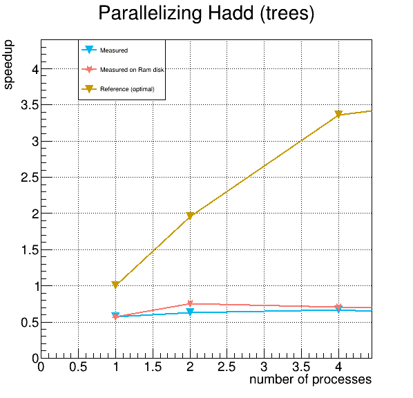
Figure 7.3: Speed up obtained when merging in parallel with hadd 48 ROOT files containing TTrees, measured both from disk and from a RAM disk, against the theoretical reference.
The results obtained, shown in Figure 7.3, are discouraging in both cases, displaying a similar undesired slowdown instead of the speed up we were hoping for. Without changing the original user interfaces we can provide remarkable speed up when merging histograms, only by applying a parallel MapReduce pattern to hadd. However, while our implementation shows significant acceleration gains when merging histogram files, it does not perform so well when merging trees.
This parallelization has also been attempted in the multithreaded execution policy, but we have failed to obtain results due to non-thread-safe invocations on global variables required by ROOT's memory manager.
7.2 Parallel analysis in RDataFrame#
RDataFrame5 (see the ROOT article of this series) is one of the most relevant developments in the ongoing modernization effort of ROOT. One of its main features is the support for implicit parallelism6, exploiting TThreadExecutor directly, e.g. for the parallel execution of the event loop, and indirectly, when performing frequent operations that support implicit multithreading (IMT) and rely on TThreadExecutor for executing their operations concurrently (e.g. when reading in parallel from a TTree).
RDataFrame introduces a new programming paradigm in ROOT that reduces code complexity by designing its interfaces in a user-friendly way. However, with this design, RDataFrame also introduces several performance disadvantages as a tradeoff for the easier programming model and its PyROOT implementation. This is the case of the non-negligible overhead due to the extensive use of JIT-compiling, or the cost inherent to the expression of the analysis in a modularized, higher-level way (e.g. extra function calls, allocation of partial results).
In this section, we analyze RDataFrame's convenience and benchmark its performance by porting an ad-hoc, highly optimized, parallel code to RDataFrame. This code, Totem, is used to explore an experimental model for new physics. Totem is a Monte Carlo event generator that, following this experimental model, performs a physics simulation of very forward QCD-low pT processes according to a parametric model, and writes the relevant data resulting from this simulation into histograms. It consists of a monolithic function that performs all physics-related operations, from simulation to analysis, and the generation of the resulting histograms. Parallelism is implemented by explicitly managing POSIX threads. Despite its complexity, Totem exhibits remarkable performance and scalability, as it has been designed, from inception, for execution in highly parallel architectures.
Porting this code to RDataFrame offers the following advantages:
-
Implicit parallelism: Instead of managing the threads directly through POSIX directives, RDataFrame's support for implicit multithreading allows the user to benefit from parallelism while writing (thread-safe) sequential code. In addition to the performance boost provided by RDataFrame, the user benefits from the growing number of operations in ROOT that support an IMT-based parallel mode.
-
Declarative and functional programming model: Instead of dealing with the details of its computation, users express their analyses with RDataFrame in terms of chained transformations and actions; that is, they describe which operations the analysis is composed of, instead of expressing how to perform these operations.
-
Cleaner code: Due to its functional programming model, RDataFrame increases code modularity by factoring transformations and actions out of the event loop.
-
Lazy, efficient evaluation: The processing of the graph is deferred to the first access to one action result. This is especially convenient with RDataFrame's organization of transformations and actions in a computational graph, which allows us to reuse the results from shared nodes of the graph.
As Totem's code was developed in a previous version of the software (ROOT 5), we proceed with a two-step translation, guaranteeing reproducibility after each step. First, we port the code to ROOT 6, identifying and refactoring the event loop into a single-event evaluation lambda, and relying on TThreadExecutor for its parallelization, avoiding thread-locality and simplifying the programming model by removing all thread management directives. The second step requires isolating the simulation from the analysis, encapsulating the former into a single-event evaluation lambda, and expressing the latter by means of RDataFrame, from the execution of the event loop, to the filling of the final histograms.
The original, complex code of Totem and the explanation of the physics behind it are outside of the scope of this article. However, it is helpful to examine RDataFrame's version of the code to showcase its simpler and more convenient programming model.
// Data structure to encapsulate the results to return from the simulation
class collisionData {
public:
   collisionData() {}
   collisionData(bool hC, Double_t &r, Double_t &w, Double_t &f):
                 hasCollided(hC), roffset(r), wevent(w), fr(f) {}

   bool hasCollided = false;
   Double_t roffset{};
   Double_t wevent{};
   Double_t fr{};
};

// Physics simulation.
// The data filtering and histogram generation with the results has been
// factored out, leaving the most fundamental operations on events.
auto collideOps = [&](unsigned int slot) {
   // ....
   // intensive physics computations
   // ....
   return collisionData(hasCollided, roffset, wevent, fr);
};

// Enable implicit multithreading
ROOT::EnableImplicitMT();

// Helpers
auto hasCollided = [](const bool &hasCollided) { return hasCollided; };
auto hasNotCollided = [](const bool &hasCollided) { return !hasCollided; };

// Initialize an empty dataframe with nEvents rows
ROOT::RDataFrame d(nEvents);

// Define the new per-event variables from the results obtained per-event
auto d2 = d.DefineSlot("collisionData", collideOps)
           .Define("hasCollided",
                   [&](const collisionData &colData) { return colData.hasCollided; },
                   {"collisionData"})
           .Define("roffset", [&](collisionData &colData) { return colData.roffset; },
                   {"collisionData"})
           .Define("wevent", [&](const collisionData &colData) { return colData.wevent; },
                   {"collisionData"})
           .Define("fr", [&](const collisionData &colData) { return colData.fr; },
                   {"collisionData"});

// Generate 1D and 2D histograms to visualize the results.
auto notCol = d2.Filter(hasNotCollided, {"hasCollided"});

auto helast = notCol.Filter([](const double &offset) { return offset < 1.01; }, {"roffset"})
                     .Histo1D<double>(TH1D("helast", "elastic collisions in proton range",
                                           100, distmin, 1.01),
                                      "roffset");
auto hfr = notCol.Histo1D<double>(TH1D("hfr", "p-p elastic", ntbins, tbins),
                                   "fr", "wevent");
auto hfr1 = notCol.Filter([](const double &offset) { return offset < 1.01; }, {"roffset"})
                   .Histo2D<double>(TH2D("hfr1", "hfr1", 100, 0, 0.5, 100, distmin, 0.7),
                                    "fr", "roffset", "wevent");
auto hfr2 = notCol.Histo2D<double>(TH2D("hfr2", "hfr2", 100, tmin, tmax, 100, distmin, 1),
                                    "fr", "roffset", "wevent");
auto hcoll = d2.Filter(hasCollided, {"hasCollided"})
               .Filter([](const double &offset) { return offset < 1.01; }, {"roffset"})
               .Histo1D<double>(TH1D("hcoll", "inelastic collisions in proton range",
                                     100, distmin, 1.01),
                                "roffset");
Listing 7.2: RDataFrame implementation of Totem. Lines 17-22 (original numbering) define the lambda encapsulating the Monte Carlo simulation of a single event, whose body has been omitted for irrelevance to the example; it returns, in the collisionData struct declared above it, the relevant data for the subsequent analysis. Enabling implicit multithreading turns the following event loop and histogram generation into a parallel operation without any explicit thread management.
Where possible, we maintained the original names of the variables. The lambda encapsulating the Monte Carlo simulation of a single event returns, encapsulated in the collisionData structure, the relevant data for the subsequent analysis. Enabling the implicit multithreading mechanisms in ROOT is all it takes for the automatic multithreaded parallelization of RDataFrame to kick in.
RDataFrame's dataset can be pictured as a table, where each row represents an entry of the columnar data. In this case, we initialize a new RDataFrame of nEvents (entries or rows of the data frame), and the subsequent chain of Define calls executes the Monte Carlo simulation event loop in parallel and stores the relevant quantities resulting from it in new defined variables (columns of the data frame). Finally, we perform our analysis, expressing it functionally and declaratively, in terms of chained actions and transformations. For each one of the final results (histograms), we apply first, as transformations, one or more filtering operations on the data and then, as actions, the generation of each one of the resulting one- or two-dimensional histograms.
The evaluation of the event loop in RDataFrame is performed lazily: the first time we access a result from an action of the computational graph, RDataFrame proceeds to the evaluation of the graph for all previously booked results. However, after an event loop, in case we add another result and trigger another event loop, all parts of the graph that are necessary for the generation of these results are re-evaluated. This affects directly the way we express our analyses, as an inefficient booking of the results may result in unnecessary computational redundancy—for instance, booking an additional, unrelated result after already triggering one event loop may force the re-evaluation of shared upstream transformations that had already been computed, a redundant evaluation that could be avoided by booking every result before accessing any of them.
We benchmark the performance of both versions of Totem in two highly-parallel computers. The first benchmarking machine is an Intel Xeon E5-2683 v37 server composed of two NUMA domains with 14 physical cores and 28 logical threads each at 2.00 GHz with 32 GB of RAM per NUMA node. The second, more extreme, many-core computer is an Intel Xeon Phi 72108 server composed of two sockets with 64 cores each at 1.3 GHz (supporting hyperthreading) and 110 GB of RAM in total. In order to avoid confusion, we refer to this computer by its former code name: Intel Knights Landing (KNL). The times obtained have been measured with the standard high resolution clock of C++, each one averaged over several executions.
| Threads | RDataFrame (s) | Original (s) | Ratio |
|---|---|---|---|
| 1 | 2932.95 | 2919.44 | 0.99 |
| 10 | 297.66 | 304.75 | 1.02 |
| 20 | 151.32 | 151.64 | ≈1 |
| 30 | 117.38 | 116.55 | 0.99 |
| 40 | 96.16 | 96.49 | ≈1 |
| 50 | 81.75 | 81.66 | ≈1 |
Table 7.2: Execution time of Totem for a simulation of 36000 events on the Intel Xeon server.
| Threads | RDataFrame (s) | Original (s) | Ratio |
|---|---|---|---|
| 1 | 13842.96 | 14011.58 | 1.01 |
| 16 | 887.49 | 869.35 | 0.98 |
| 32 | 468.13 | 448.58 | 0.96 |
| 64 | 253.55 | 237.56 | 0.94 |
| 96 | 188.66 | 184.81 | 0.98 |
| 128 | 156.21 | 151.88 | 0.97 |
| 146 | 144.21 | 149.09 | 1.03 |
| 164 | 132.49 | 146.78 | 1.11 |
| 182 | 123.58 | 151.10 | 1.22 |
| 200 | 120.84 | 159.61 | 1.32 |
Table 7.3: Execution time of Totem for a simulation of 36000 events on the Intel Knights Landing (KNL) server.
We observe near-identical performance between the execution time of the original code and RDataFrame's implementation on the Xeon server, with the ratio between the two hovering around 1 regardless of the thread count. Instead, the KNL benchmark exhibits a remarkable difference in scalability in favour of RDataFrame when approaching extreme levels of parallelism: from 146 threads onward, the ratio climbs well past 1, reaching 1.32 at 200 threads, meaning RDataFrame's version runs noticeably faster than the original, hand-tuned POSIX-threads code. RDataFrame, while offering a more general, convenient and user-friendly way to express the analysis, not only matches the performance of the original ad-hoc code but improves its scalability in many-core architectures.
7.3 Vectorization of mathematical formulas compiled at runtime#
TFormula, the formula class in ROOT, is the perfect candidate to benefit from vectorization. TFormula translates user-defined formulas, expressed as a string, by compiling them into C++ code at runtime, exploiting JIT compilation with Cling. In addition to simple variables and C++ code supported by the standard, TFormula supports ROOT-defined and user-declared functions registered in a list of global functions kept by ROOT, e.g. a function defined with a TF1. Moreover, TFormula provides automatic translation of the most common functions used in HEP analysis into their C++ inline representation, such as "gauss" (Gaussian distribution) or "landau" (Landau distribution). TFormula is an important component of ROOT, and it is used extensively, from the analysis evaluation in TTree::Draw() to the definition of TF1 functions.
Vectorization is implemented in TFormula by compiling the formula variables into ROOT's SIMD types (ROOT::Double_v) and relying on VecCore's backend to perform the SIMD operations (see the Data-level parallelism article of this series). TFormula's list of automatically translated functions has been extended to provide automatic translation for functions with a VecCore implementation (e.g. exp translates into vecCore::math::Exp).
The following listing displays a code example for the declaration of a formula. The first line creates the function "Signal" from a formula and registers it in the global list of ROOT; from this moment, "Signal" is available for usage in other formulas. The second statement performs the same operation for a different formula, "Background". The declaration of "FormulaV" showcases the usage of user-declared functions once they have been registered, creating the new function from a formula composed of the addition of the previous two declared functions. The only significant difference between this code and that for a scalar formula is the final call declaring the function to be vectorizable—a change in the nature of the data the formula accepts that is still possible at this stage because the JIT compilation of the formula occurs upon invocation instead of on declaration.
auto fSignal = new TFormula("Signal", "[0] * (-(x + (-130.)) * (x + (-130.)) / 2)");
auto fBackground = new TFormula("Background",
                    "[0] * (-([1] * (x * (0.01)) - [2] * (x * (0.01)) * (x * (0.01))))");

auto fFormula = new TFormula("FormulaV", "Signal+Background");
fFormula->SetVectorized(true);
Listing 7.3: TFormula declaration for a signal-plus-background model, with vectorized evaluation enabled on the combined formula.
We propose three different cases, or functions, to benchmark the performance of vectorization in TFormula. Case 1 evaluates a function composed of the sum of a signal given by a Gaussian distribution centered on 130 with variance 1, and a background given by an exponential function with a polynomial exponent—this is the function declared from a formula in Listing 7.3. Case 2 evaluates a similar function that removes the exponential calls. Case 3 evaluates a simple polynomial.
For a more extensive comparison, we implement each one of the cases as a free function; as a TF1 wrapping a free function; as a TFormula; and as a TF1 wrapping a ROOT formula. We compiled these benchmarks with Apple Clang 9.1.0 and AVX2 as the set of instructions, on an Intel Core i5-4278U9 processor with 4 cores at 2.6 GHz and 8 GB of RAM.
| Case | Implementation | Scalar (ns) | Vectorized (ns) | Speed up |
|---|---|---|---|---|
| 1 | Free function | 11.6 | 12.1 | 0.96 |
| TF1 (free function) | 28.5 | 13.2 | 2.15 | |
| Formula | 22.9 | 12.8 | 1.79 | |
| TF1 (formula) | 26.2 | 13.1 | 2.00 | |
| 2 | Free function | 1.89 | 0.541 | 3.50 |
| TF1 (free function) | 8.48 | 2.39 | 3.55 | |
| Formula | 22.8 | 13.0 | 1.76 | |
| TF1 (formula) | 27.0 | 12.9 | 2.10 | |
| 3 | Free function | 1.50 | 0.467 | 3.22 |
| TF1 (free function) | 7.91 | 1.93 | 4.09 | |
| Formula | 22.1 | 8.36 | 2.64 | |
| TF1 (formula) | 24.6 | 8.50 | 2.90 |
Table 7.4: Execution time and speed up, normalized to the size of the data, for the scalar and SIMD evaluation of each of the three cases over one data point, implementing each one as a free function, as a TF1 wrapping a free function, as a TFormula, and as a TF1 wrapping a ROOT formula.
The results exhibit a disparity in results for TFormula when vectorizing. While we expect TFormula to perform worse than a free function due to the overhead and extra levels of indirection introduced by the JIT compilation, the differences in speed up indicate a suboptimal performance of the formula code, reaching in Case 2 a divergence of 2× in favour of the free function vectorization with VecCore. TF1, on the other hand, performs as expected, experiencing little overhead when evaluating short functions—despite the introduction of virtual calls and extra levels of indirection—consistently roughly doubling (or more) its throughput once vectorized. Notably, autovectorization also affects the results in Case 1, making the vectorized implementation of the free function slightly slower than the scalar one, as the compiler was already able to autovectorize part of the scalar version.
Conclusions#
The three independent studies presented in this article confirm, on real and varied workloads, the value of the parallelization work described throughout this series. Parallelizing hadd with a MapReduce pattern, without touching its user-facing interface, yields large speed ups when merging histogram files, although the same approach falls short for TTrees, where the sequential I/O optimizations already in place are harder to beat. Porting a highly-tuned, explicitly multithreaded physics analysis to RDataFrame matches the performance of the original code on a regular multicore server, and surpasses it on an extreme many-core architecture, all while trading low-level thread management for a declarative, more maintainable programming model. Finally, vectorizing TFormula via VecCore delivers consistent gains for TF1-wrapped formulas, even if the overhead of the JIT-compiled formula machinery keeps bare TFormula evaluation from fully reaching the speed ups observed for free functions.
-
Dean, J., & Ghemawat, S. (2008). MapReduce: simplified data processing on large clusters. Communications of the ACM, 51(1), 107-113. ↩︎
-
Guiraud, E., & Ganis, G. (2015). Enhancements to Multiprocessing in ROOT. link ↩︎
-
Guiraud, E., Naumann, A., & Piparo, D. (2017). TDataFrame: functional chains for ROOT data analyses. link ↩︎
-
Canal, P., Ganis, G., Guiraud, E., Mato Vila, P., Moneta, L., Piparo, D., Tejedor, E., & Valls Pla, X. Expressing Parallelism in ROOT. 22nd International Conference on Computing in High Energy and Nuclear Physics, Journal of Physics: Conference Series, IOP. ↩︎