SIMD in ROOT: introducing VecCore
This article is part of a series that I'm slowly publishing, and it still has several broken links referencing unpublished articles.
In addition to task-level parallelism, where we distribute the workload between the multiple cores or processors of a system, we can further parallelize the computations performed in each core by taking advantage of data-level parallelism. Modern architectures support different SIMD instruction sets that enable us to capitalize on the larger CPU registers existing in current computers to perform simultaneous operations on multiple data elements.
This article describes the work done to introduce data-level parallelism in the mathematical libraries of ROOT. Section 5.1 discusses the concept of vectorization and describes some of its common pitfalls. Section 5.2 introduces VecCore, the vectorization library we introduce in ROOT to implement SIMD operations, and benchmarks its performance by exploiting SIMD operations to generate Julia sets. We use this same benchmark in Section 5.3, to analyze the performance of the support for VecCore types evaluation in TF1, the bounded function class in ROOT.
5.1 Vectorization#
Data-level parallelism is achieved in ROOT by exploiting SIMD operations on arrays of data.
Vectorization allows the loading of several values of a specific type in an SIMD array and the activation of the same operation on them simultaneously. The number of elements that we can operate with at the same time will depend on the set of instructions supported by the architecture and the data type of the elements. Table 5.1 provides a relation of sizes for the most common data types and sets of instructions on Intel x86 architectures.
| Instructions | Array size (bit) | int (16 bit) | float (32 bit) | double (64 bit) |
|---|---|---|---|---|
| SSE | 128 | 8 | 4 | 2 |
| AVX2 | 256 | 16 | 8 | 4 |
| AVX512 | 512 | 32 | 16 | 8 |
Table 5.1: Relationship between the set of SIMD instructions, the size of the SIMD array supported and the number of elements of each type that fit in it.
For all these benefits, vectorization does not come without pitfalls. Among the problems that may arise when vectorizing, such as wrong type conversions or non-aligned memory, one of the most serious is branching. In the traditional scalar case, a control flow instruction chooses which branch of the code to select based on a condition, and then executes only the set of instructions corresponding to that branch. In SIMD programming, these control flow operations require performing the computations on all branches and, afterwards, assigning their results per element position, depending on a mask filter created when evaluating the condition on an SIMD array. This is a common operation that can have a strong negative impact on performance. Figure 5.1 illustrates these flows for conditional branching.
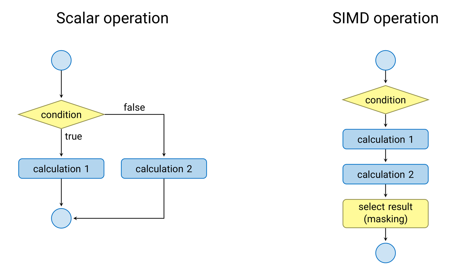
Figure 5.1: Comparison of the conditional branching flow between traditional scalar instructions and SIMD instructions.
In addition to these problems inherent to vectorization, there is the question of usability. Vectorization is usually expressed with compiler intrinsics, which do not expose the most user-friendly interfaces. Libraries such as Vc1 or UME::SIMD2, while different in concept, improve the readability and usability of the code by abstracting these instructions and providing a more familiar and user-friendly interface for the developer. The vectorization library used in ROOT, VecCore, goes one step further and provides an abstraction over these two libraries.
Despite the disadvantages, vectorization offers enough performance benefits to prefer it over scalar operations.
5.2 VecCore#
VecCore3 provides efficient vectorization on a variety of platforms by offering an abstraction layer on top of the libraries Vc, UME::SIMD and the language extension CUDA4.
These three libraries are supported as optional backends as well as a fallback scalar one in case SIMD operations are not available. The users will make their choices depending, for example, on system availability, performance or simple preference.
VecCore allows the development of architecture-oblivious code that maps to the appropriate backend specific types, methods and instructions. Figure 5.2 displays graphically the most important and recurrent of these instructions, while Listing 5.1 presents its code API.

Figure 5.2: Graphical depiction of the VecCore API.
Get and Set allow safe read/write access to the individual elements of the SIMD array. Given an iterable container of indices, Scatter will distribute the elements of the SIMD arrays pointed by those indices, while Gather will access the elements referenced by the given indices of the data array and load them into the SIMD array. MaskedAssign and Blend depend on the concept of masking.
A boolean mask is generated when a condition is applied to an SIMD array. This mask signals which elements of the array fulfill the condition and which do not. MaskedAssign takes the generated mask, a value, and the destination SIMD array as input, and stores the value in the positions given by the true values in the mask. If the value is an SIMD array, the assignment is done element-wise. Blend performs the same operation but takes as an input another value that will be assigned to the elements that do not meet the condition.
namespace vecCore {

template <typename T> struct TypeTraits;
template <typename T> using Mask   = typename TypeTraits<T>::MaskType;
template <typename T> using Index  = typename TypeTraits<T>::IndexType;
template <typename T> using Scalar = typename TypeTraits<T>::ScalarType;

// Vector Size
template <typename T> constexpr size_t VectorSize();

// Get/Set
template <typename T> Scalar<T> Get(const T &v, size_t i);
template <typename T> void Set(T &v, size_t i, Scalar<T> const val);

// Load/Store
template <typename T> void Load(T &v, Scalar<T> const *ptr);
template <typename T> void Store(T const &v, Scalar<T> *ptr);

// Gather/Scatter
template <typename T, typename S = Scalar<T>>
T Gather(S const *ptr, Index<T> const &idx);

template <typename T, typename S = Scalar<T>>
void Scatter(T const &v, S *ptr, Index<T> const &idx);

// Masking/Blending
template <typename M> bool MaskFull(M const &mask);
template <typename M> bool MaskEmpty(M const &mask);

template <typename T> void MaskedAssign(T &dst, const Mask<T> &mask, const T &src);
template <typename T> T Blend(const Mask<T> &mask, const T &src1, const T &src2);

} // namespace vecCore
Listing 5.1: VecCore API.
Listing 5.2 shows how the branching operations described in Figure 5.1 are applied using VecCore.
// ROOT::Double_v is the new VecCore based
// double SIMD type integrated in ROOT
ROOT::Double_v x_v, res_v, var1_v, var2_v;
double x, res, var1, var2;

// (.....)

// Case 1: Assigning rvalues if condition is fullfilled
double res = x<0.? 1.: 2.;
vecCore::Blend(res_v, x_v<0.0, 2);

// Case 1: Assigning variables element-wise if condition is met
double res = x<0.? var1: var2;
vecCore::Blend(res_v, x_v<0.0, var1_v, var2_v);

// Case 3: Only updating elements of the SIMD array that pass the condition
if(x<0.){
   res+=var1;
}
vecCore::MaskedAssign(res_v, x_v<0., res_v + var1_v);
Listing 5.2: Comparison of the expression of branching conditions between the scalar case and using VecCore.
In addition to the described API, VecCore offers vectorized mathematical functions and some other interesting utilities such as the Load method, which deals with problems caused by reading from unaligned memory, and safe type castings.
ROOT defines new VecCore-based SIMD array data types, e.g. ROOT::Float_v or ROOT::Double_v, representing double and single precision SIMD vectors respectively.
Performance analysis: generating Julia sets. We next leverage the generation of Julia sets5 as a benchmark to evaluate the performance of vectorization with VecCore.
Julia sets are most popularly represented as complex quadratic polynomials. The Julia set we benchmark is composed of a fixed subset of image points (x, y) on the complex plane z = x + iy, z ∈ ℂ, for which we compute the series zn+1 = zn2 + c, c ∈ ℂ, -2 ≤ zn ≤ 2, where z0 = xj + iyj, and x and y are the coordinates of the point j in the complex plane, and the series is evaluated until divergence (values of zn out of bounds) or until zN, with N being the maximum number of evaluations set by the user to approximate the progression in the bounded case. We obtain a different Julia set approximation for each value of the complex constant c.
The code for generating a fractal image related to the Julia set with any library other than the standard one iterates, for each pixel, the series above until either it diverges or the maximum number of iterations is reached, storing the resulting step count as the pixel value. Listing 5.3 implements a version of the same code adapted for vectorization using VecCore: instead of computing one pixel at a time, we advance an entire SIMD lane of pixels together, using MaskedAssign to freeze the lanes that have already diverged while the remaining ones keep iterating, and MaskEmpty to detect when every lane in the array has terminated. The value of each pixel in the final image is given by a function of the number of steps taken by the progression on each point until termination, for both the set of points within our approximation of the Julia set and the ones for which the series diverged. We refer to these images as a representation of the Julia set, despite including values outside of the set.
Listing 5.3: VecCore based implementation of a Julia set generator. This implementation can be executed on any backend supported by VecCore, from the Scalar backend to Vc or UME::SIMD, and it can target any set of SIMD instructions supported by the architecture it executes on.
Benchmarking the evolution of Julia sets. From the recurrence above we infer that the time needed to generate different Julia sets from the same initial subset of points in the complex plane varies significantly with the value c. For this reason, we consider it interesting to evaluate the performance of vectorization with the evolution of the fractal image, that is, the Julia sets generated with different values for the complex constant c.
To do this, we represent c as a complex number in polar form, i.e. c = b·eiα, where b ∈ ℝ and α is the angle parameter in the interval [0, 2π). If we fix the value of b, e.g. to b = 0.7885, and approximate the series by restricting the maximum number of evaluations to N = 100, we observe the evolution of the fractals given by the Julia sets defined by the progression zn+1 = zn2 + 0.7885eiα, -2 ≤ z ≤ 2, α ∈ [0, 2π), n ≤ 100.
The following measurements have been taken in an Intel Core i7-4790 desktop server with 4 physical cores (8 logical threads) at 3.6 GHz and 8 GB of RAM, executed with AVX2 as SIMD instruction set and compiled with gcc 7.
The execution time measured for a continuously increasing α exhibits high volatility based on the value of α, independently of the backend of choice. These measurements also reveal that Vc outperforms UME::SIMD in any benchmarked type and that, while vectorization always provides better times, the scalar backend displays minimal performance penalty overall and even occasionally improves the time obtained when evaluating the base types, an effect we attribute to auto-vectorization performed by the compiler on the base-type code.
The speed ups stay below the ideal ones and, although they improve occasionally in several spikes that match those of the execution time, they are greatly influenced by the backend of choice. If we compute the speed up of these results with respect to the time obtained for the base types without allowing auto-vectorization, we observe that Vc considerably outperforms UME::SIMD as a backend in both cases (Table 5.2). In addition, VecCore's scalar backend now improves the time obtained with the base types, although it does not match the autovectorization offered by the compiler, except on the spikes. Curiously, it is in the same spikes that we obtain the best vectorization for any of the other backends. This seems to indicate that the vectorization requires a greater amount of work to yield noticeable benefits. If we plot the fractal picture, i.e. the Julia set generated, for the value of the angle α corresponding to each of the local maximums observed, we observe that these images have a sizeable black area. We call this the convergence area, that is, an area composed of points that did not diverge before reaching the Nth step in the series progression (our approximation to the theoretical notion of a Julia set).
| float | double | |||
|---|---|---|---|---|
| Backend | UME::SIMD | Vc | UME::SIMD | Vc |
| Reference | 8 | 8 | 4 | 4 |
| Max. speed up | 6 | 6.17 | 1.75 | 2.84 |
| Min. speed up | 2.75 | 3.52 | 1.27 | 2.02 |
| Avg. speed up | 3.45 | 4.36 | 1.51 | 2.34 |
Table 5.2: Comparison of the maximum, minimum and average speed ups obtained with respect to the ideal ones (Reference) for the Vc and UME::SIMD backends of VecCore evaluating in the AVX2 instruction set.
When vectorizing the generation of Julia sets, we attribute the improved speed up to the existence of large uniform areas. In contrast with the N evaluations reached by the points within the convergence area, the points that diverge (i.e. reach out of bounds values, in this case outside the interval [-2, 2]) require a heterogeneous number of evaluations of the series progression. In terms of computation, this is related to the conditional branching problem introduced in Section 5.1: let S be an SIMD array fitting 4 integers, and let x⃗ be an array of integer data of the same size as the SIMD array, in which processing each component takes 10, 20, 80 and 35 evaluations respectively. In the scalar case the total number of evaluations required is the sum of the evaluations required for each element, 10+20+80+35 = 145. In the vectorized case the SIMD array is evaluated as a whole as many times as the element that requires the most evaluations, that is, 80. In this example we obtain a speed up of 145/80 = 1.81, when the ideal one (i.e. each element requires the same number of evaluations) would be 4. A homogeneous area in the image indicates that the pixels within its borders take a similar number of evaluations and, as a consequence, avoid the problem of conditional branching. Heterogeneous areas may cause the fluctuations in execution time and speed up we observe. However, after analyzing the homogeneity of the images and computing the potential speed up loss caused by branching for several values of α, it becomes clear that branching only affects the speed up in a minimal way in this case, almost negligible with respect to the results obtained.
If we benchmark the code line by line, and analyze the assembly instructions, we can deduce that the vectorization libraries themselves are responsible for the suboptimal speed ups. The implementation of these libraries, and especially the SIMD intrinsics chosen to implement the abstracted operations, might impact performance considerably. For example, in the implementation of the initialization of the mask in Vc, and probably as a compromise to offer a user-friendly interface, the code loops through the SIMD array, assigning the initialization value element by element. These instructions are scalar instead of packed. This occurs in UME::SIMD as well. Due to the particularities of its design, UME::SIMD emulates scalar instructions instead of using vector operations more frequently than Vc. Furthermore, the out-of-order execution of the processor might be able to process and parallelize scalar operations more efficiently at instruction level.
In addition, the architecture we execute on may attenuate the differences in speed up even more, especially with respect to instruction-level parallelism. For example, Intel's Skylake architecture offers a throughput of 3 instructions per CPU cycle for the AVX2 8-bit integer addition instruction, improving the rate obtained on the Broadwell and Haswell architectures, which both sit at 2 instructions per cycle for the same operation.
Compiler comparison. A conspicuous result from the previous benchmarks is the difference in speed up between Vc and UME::SIMD. One of the most plausible reasons for this considerable gap in performance is that UME::SIMD is a library that has been optimized for its use in combination with icc instead of gcc. That is, the implementation of the vectorization directives in each library used as a backend for VecCore may be optimized for a concrete compiler.
Therefore, it is interesting to measure the difference in performance of these libraries when relying on different compilers, in order to make an informed decision about the combination of VecCore backend and compiler that provides the best performance. We compare the speed up for both float and double types in AVX2 SIMD arrays for three main compilers (gcc, icc and clang), measured on the same Intel Core i7-4790 desktop server, without task-level parallelism being exploited.
We observe that Vc generates more efficient SIMD instructions when compiling with gcc and clang, while UME::SIMD displays better results with icc than gcc. In particular, Vc shows a considerably higher speed up in the double precision case for both gcc and clang in comparison with any other combination.
If the best option were to be selected in terms of speed up, Vc and gcc would be the combination of choice, closely followed by Vc plus clang. However, this deduction is based on a wrong premise, as the speed ups are computed as a factor of the sequential execution compiled by the same compiler. Therefore, we cannot base our decision on the speed up metric alone.
Instead, we must consider the absolute execution time. Comparing the different execution times observed with our benchmark code for an increasing α in the interval [0, 2π), we conclude that the best absolute choice is to compile Vc with gcc, while the worst one is to compile UME::SIMD code with clang. In general, we note that Vc reduces the time obtained by UME::SIMD independently of the compiler.
Efficiency of Julia set generation for different sets of instructions. Finally, we measure the efficiency of our implementation when executing VecCore's vectorized backends on different sets of SIMD instructions. For a more complete picture, we execute our benchmark on a machine that supports SSE2, AVX2 and AVX512 as sets of instructions, an Intel Xeon Phi 7210 server composed of two sockets with 64 cores each at 1.3 GHz (supporting hyperthreading) and 110 GB of RAM in total. The benchmark is executed in the quadrant execution mode of the Xeon Phi, and it has been compiled with icc 17 (the only compiler yet supporting the AVX512 set of instructions).
In general, the results exhibit less fluctuation and volatility on this platform (Xeon Phi) than on the previous servers.
One of the first things we notice is that Vc does not have a proper AVX512 implementation and falls back to AVX2. Therefore, the times and speed up obtained by Vc for both the AVX2 and the AVX512 sets of instructions are similar. While executing with AVX2, Vc improves the results of UME::SIMD for the double case, but underperforms with float. The inverse occurs when executing with SSE2, with Vc significantly improving the results attained by UME::SIMD, which shows a slight slowdown with respect to the base type execution in this case. Finally, UME::SIMD displays high scalability between the three instruction sets, and the support of the AVX512 SIMD instruction set renders it the most convenient backend when executing on platforms that support it.
As a final remark, the speed up obtained with the combination of UME::SIMD and AVX512 is the best we have recorded for any benchmark, but looking at the execution time, we can assert that this platform's processor frequency is too slow to make it the preferred option.
5.3 Generating Julia fractals with TF1#
We benchmark again the generation of Julia sets, this time with a constant c = 0.285 + 0.01i, using the new ROOT SIMD types, concretely ROOT::Double_v, and the interfaces we adapted for vectorization. For this, we use TF1, the ROOT class representing a one dimensional function defined between lower and upper limits. TF1 is a wrapper over a user-specified function that extends its functionality to adapt it to ROOT's interfaces and conforms a fundamental class in ROOT. It is also the base class for the multidimensional function classes (TF2, TF3), and it is leveraged with frequency, from fitting (as it can be parameterized) to graphics display.
Unlike other classes, such as those that define the fitting interfaces, TF1 is exposed to the user for direct manipulation. For this reason, and to maintain backwards compatibility, instead of templating the class, we template the necessary class members to process the new vectorized types. This makes existing code available for vectorization by adapting the user function to operate on ROOT::Double_v.
In addition, we developed TF1 further with new features such as new constructors for std::function types and the possibility to evaluate over scalar data types (double) when the function that TF1 has been built on is vectorizable. In this case, we fill the entire SIMD array with the scalar value, operate with it, and return only one of the (identical) values of the resulting SIMD array.
Our benchmark also serves to measure the adaption of a user function with more than two parameters to the TF1 interfaces. TF1 is a parametric function with strict interfaces, allowing as its only parameters a pointer to the data and a pointer to the parameters needed for the evaluation of the user function. This limitation is frequently overcome by wrapping the user function in a C++ functor, packing the parameters in an array of double when calling the TF1, and unpacking them after forwarding the call to the user provided functor. This operation adds a slight overhead in the packing/unpacking process and to the call forwarding.
The benchmark was run on an Intel Core i7-4790 desktop server with 4 physical cores (8 logical threads) at 3.6 GHz and 8 GB of RAM, executed with AVX2 as set of SIMD instructions and compiled with gcc 6.2. The functor adaption and TF1 wrapping adds a small overhead in all cases, and VecCore's scalar backend essentially matches the performance attained by the original code, including performing several masking operations as a consequence of conditional branching (Section 5.1). Finally, we observe a fair speed up when vectorizing, considering the complexity of the problem at hand: the scalar evaluation of the functor-wrapped function takes around 136 ns per call, VecCore's scalar backend matches it at around 131 ns, and switching to the vectorized ROOT::Double_v backend brings the cost down to around 52 ns per call — evaluating several points of the fractal in the time it previously took to evaluate one.
We further benchmark the performance of TF1 in the Putting ROOT's parallel tools to the test article of this series, where we compare the single call performance of TF1 built with a free function and TFormula, the formula class in ROOT, with their vectorized counterparts.
5.4 Conclusions#
We introduced data-level parallelism in ROOT by capitalizing on the advantages offered by the VecCore library and its backends in terms of programming model and performance. By offering an extra abstraction layer on top of its exchangeable backends, VecCore provides efficient vectorization with an improved yet simpler programming model that, among other benefits, allows for better portability with the development of architecture-oblivious code.
We benchmarked VecCore's performance extensively with a complex example, the computation of different Julia sets. We evaluated the generation of Julia sets on two different floating point types, float and double; two different computers, a desktop server and a Xeon Phi; two different VecCore backends, Vc and UME::SIMD; three different compilers, icc 17, gcc 7.2 and clang 5; and three different instruction sets, SSE2 (desktop server and Xeon Phi), AVX2 (desktop server and Xeon Phi) and AVX512 (Xeon Phi).
In all cases, VecCore exhibits suboptimal speed ups due to the nature of the benchmark, with gcc performing better than icc or clang. We demonstrate that Vc outperforms UME::SIMD in almost all scenarios, but the latter supports AVX512, which is not the case for the former. Finally, while the highest speed ups are obtained with AVX512 on the Xeon Phi server, the processor frequency on this machine is not fast enough to consider this combination the best option.
In addition, we introduced two new SIMD types based on VecCore types in ROOT, ROOT::Float_v and ROOT::Double_v, for the implementation of SIMD operations in ROOT's classes. Moreover, we provided an example of the integration of VecCore within ROOT by introducing VecCore-based SIMD evaluation in TF1, the bounded function class, which is widely used in ROOT for the performance of mathematical operations. We compared the execution of a vectorized function as a free function with the same function adapted for its execution as a TF1. We demonstrate an efficient implementation of SIMD vectorization in TF1, which even with the required scaffolding, produces almost negligible overhead over the free function evaluation.
-
Kretz, M., & Lindenstruth, V. (2012). Vc: A C++ library for explicit vectorization. Software: Practice and Experience, 42(11), 1409-1430. link ↩︎
-
Karpinski, P., & McDonald, J. (2017). A high-performance portable abstract interface for explicit SIMD vectorization. In PMAM@PPoPP, 21-28. link ↩︎
-
Amadio, G., Canal, P., & Wenzel, S. (2017). root-project/VecCore: Release v0.4.2. link ↩︎
-
Nickolls, J., Buck, I., Garland, M., & Skadron, K. (2008). Scalable parallel programming with CUDA. Queue, 6(2), 40-53. link ↩︎
-
Julia set https://en.wikipedia.org/wiki/Julia_set ↩︎