ROOT
This article is part of a series that I'm slowly publishing, and it still has several broken links referencing unpublished articles.
ROOT1 is an open-source, cross-platform, object-oriented C++ framework for data analysis, conceived for the practice of High Energy Physics (HEP). Starting as a private project by Rene Brun and Fons Rademakers, ROOT has been at the heart of most HEP analyses during more than two decades, in continuous development and improvement, being in constant communication with the community, obtaining invaluable feedback, providing great toolkit support, and evolving the product according to the needs of its userbase.
ROOT experienced an early fast adoption and it was soon adopted as the official LHC analysis framework. Today, ROOT is a fundamental tool in the field of HEP, and continues to be developed as a collaboration between research institutions and particular users around the world. Every day thousands of physicists use ROOT-based applications to analyze and visualize their data. Designed for storing and analyzing exabytes of data efficiently, ROOT offers a coherent set of features oriented to HEP data analysis. One of ROOT’s most important features is the streaming of C++ classes to a compressed machine-independent file format. These C++ classes are often the ones ROOT optimizes and offers for the statistical analysis of large datasets in columnar (stored and accessed column-wise) format.
In order to perform statistical analysis, physicists have at their disposition in ROOT a considerable number of functions, methods and libraries (e.g. RooFit, RooStats) especially oriented to the most common operations in HEP, such as fitting or multivariate analysis. The results of the analysis can be visualized directly from ROOT, without the need for external libraries, and stored in high quality graphic plots in any of the most common and important formats.
The complete analysis can be developed incrementally with Cling, ROOT’s interactive interpreter, benefiting from fast prototyping and exploration of ideas. Furthermore, it can be programmed in languages other than C++ thanks to ROOT’s language bindings for R and Python. The library implementing Python bindings, PyROOT, is increasing in popularity due to the possibility to interface with widely used Python scientific libraries, such as NumPy or TensorFlow. ROOT acknowledges this by designing its new features with it in mind, e.g. RDataFrame2.
This article describes some of ROOT’s most important components. ROOT’s long-lived success and early fast adoption has been traditionally based on its highly useful features for HEP analysis, such as its interactive C++ interpreter (Section 1); its high-performant I/O (Section 2); its mathematical and statistical libraries (Section 4); and the graphic representation of the analysis (Section 6). Furthermore, ROOT now offers new exciting developments for the physicists of tomorrow, such as the new paradigm for declarative analysis, RDataFrame (Section 5); the adoption of implicit multithreaded parallelism by default (Section 3); the increasingly ubiquity of SIMD operations in Math libraries (Section 3); the possibility to perform web-based analysis with the Service for Web based ANalisys (SWAN)3; and the new redesigned interfaces for the next version of the software, ROOT 7, that are being deployed gradually into the main codebase.
1. Cling#
The ROOT userbase is mainly composed of non-expert users looking for a user-friendly and fast way to program their data analyses. Compiled languages, like C++, require investing a considerable amount of time in the compilation and linking stages, even more so in large codebases such as that of ROOT. This inconvenience makes interpreted languages (e.g. Python) more attractive when performance is not paramount for the nature of the problem at hand, e.g. for exploration of interfaces or for validating the execution of a simple instruction.
One of the main benefits offered by an interpreter is faster prototyping for Rapid Application Development (RAD)4. Prototyping allows the developer to explore ideas cheaply (reduced cost), and it is an efficient way to identify and address problems early on, to identify requirements and to estimate development costs, timescales and potential resource requirements.
In addition to reducing the time the user spends in compilation and linking, interactive interpreters allow users to explore ideas even more efficiently, using the fewest resources possible, in order to validate the ideas’ effectiveness and detect, early on, any problems in their design (such as wrong assumptions). For improved usability and user-friendliness, these interpreters adopt the read-eval-print-loop (REPL)5 environment model, providing users with an interactive environment that executes single inputs and returns the result after evaluation. In addition, a REPL interpreter usually extends the programming language by making it possible to run expressions at the global level and by implementing special commands that provide information about the current state of the environment (Reflection).
Conveniently, current compiler technology allows the emulation of interpreter behaviour in compiled languages by means of incremental compilation and hybrid compilers, that is, compilers offering hybrid compilation-interpretation and Just-InTime (JIT) compilation. To emulate interactive interpretation, the hybrid compiler translates the source code into a machine-independent, observable, intermediate representation that is compiled and executed by the JIT compiler at runtime.
In order to accelerate development speed and quality, and to help overcome the complexity of the framework and the programming language, ROOT is distributed with Cling6, a user-friendly and interactive C++ interpreter built on top of Clang and the LLVM compiler infrastructure.
The Cling interpreter is a fundamental component of ROOT that is used in four principal ways:
-
JIT compiling: ROOT makes extensive use of Just-In-Time compilation throughout its code, most commonly to simplify its programming model and its user interface. It is used, for example, for the compilation at runtime of mathematical expressions provided as a string or to compile the simplified interfaces of RDataFrame after adding its template parameters at runtime (Section 5).
-
Reflection and data-type information: Reflection, the ability of a computer program to inspect and modify its own data, is necessary for the serialization and deserialization of data classes in I/O operations. Thanks to the interpreter, ROOT is capable of retrieving information from the data types at runtime, interfacing clang through cling, to provide metadata to the write-out of the objects on disk (serialization). When reading this data from disk, the interpreter will utilize the metadata to instantiate at runtime, by jitting, the objects read from the file.
-
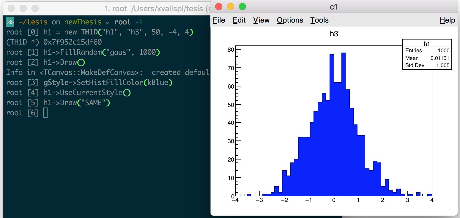
The ROOT prompt: The prompt, a REPL environment offered by the interpreter, provides the user with immediacy and interactivity one line of code at a time, making easier and faster the exploration and modification of ideas. Figure 1.1 displays two of its advantages: the value printing of C++ objects and built-in compiler diagnostics, improved from the clang ones. Figure 1.2 exemplifies how we can use the interactive interpreter to approach complex programs, such as the customization of a visualization, incrementally. By obtaining visibility into the program’s state, thanks to Cling, we benefit from immediate feedback on simple mistakes early on.
-
Support for python bindings: The interpreter provides automatic dynamic bindings between the python library (PyROOT) and the implementation of the classes in C++. It automatically generates a python wrapper over the ROOT classes allowing Python to execute C++ code without explicit development of the C++-Python bindings.
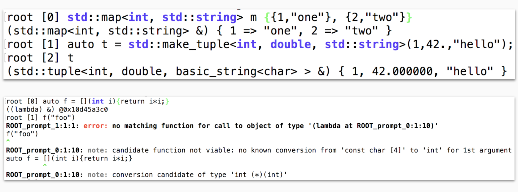
Figure 1.1: The ROOT interpreter, Cling, allows the inspection of the C++ objects and offers immediate validation of the implementations.
Figure 1.2: Cling used to approach a problem incrementally, in this case, to explore the customization of the visualization. We can modify the aspect of the default graphical representation of a histogram at runtime, without needing to compile and run again our program.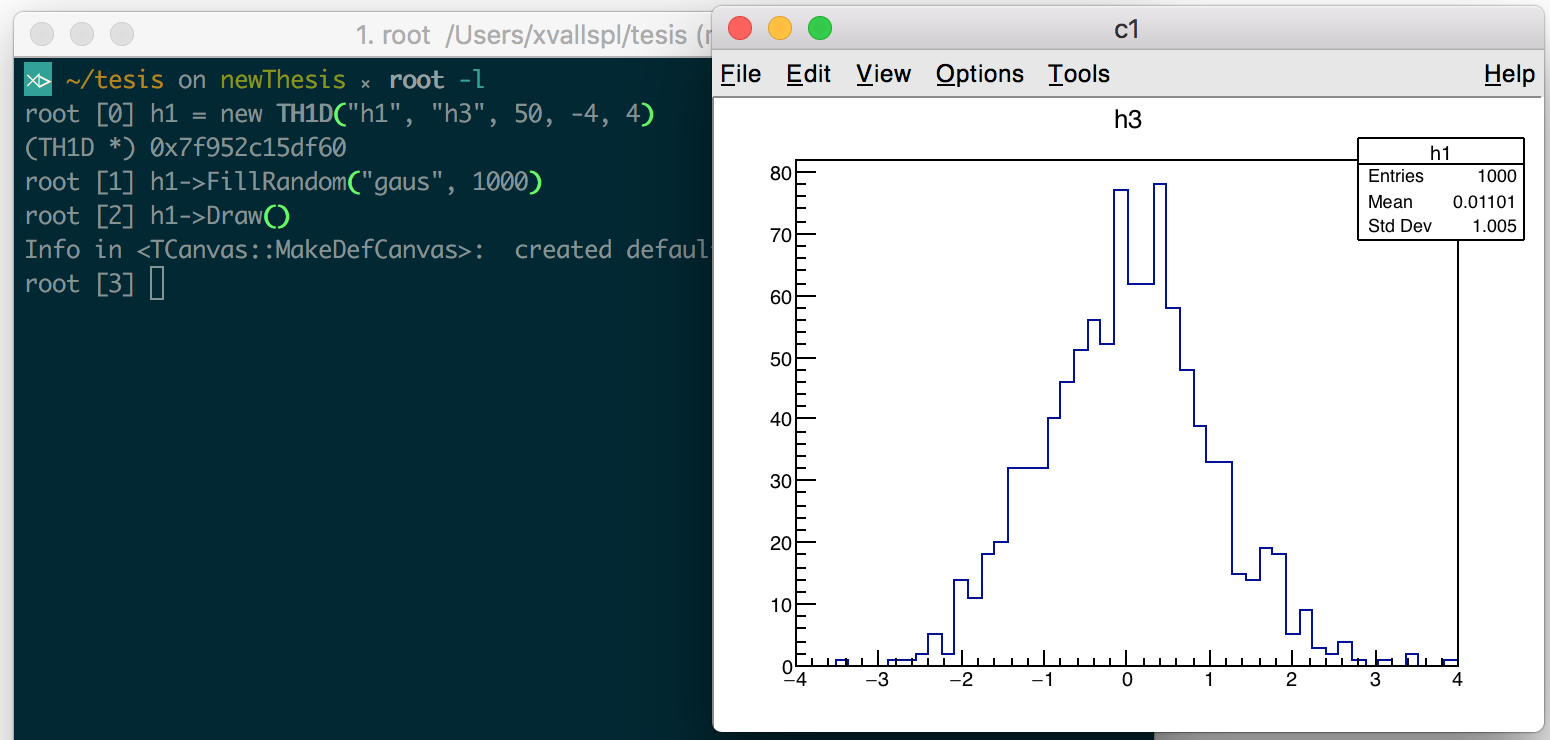
2. Input/Output#
Each year, ROOT is used to process around 50 petabytes of data. Handling such a large amount of data annually would be unreasonable without highly optimized procedures to address the limitations of the Input/Output (I/O) and data distribution systems.
For this purpose, ROOT provides a columnar file format, the ROOT file, and data structures for optimizing the reading from and writing to disk, such as the TTree, which provide the user with multiple improvements that make processing data with ROOT the most performant option available for HEP analysis. Some of these remarkable features are automatic compression and decompression, selective sparse scanning of data, directory-like storage, automatic reading of data partitioned into several files, data consistency over the lifetime of an experiment or taking advantage of the reflection capabilities of Cling to seamlessly read and write C++ objects on disk.
This section introduces the most important features in ROOT’s I/O subsystem. Section 2.1 describes the physical and logical formats of ROOT objects and Section 2.2 describes the main data structure for data representation in ROOT, the TTree.
2.1 TFile and the ROOT file format#
As introduced in Section 1, a very interesting feature that ROOT offers is the possibility to automatically store and read any C++ object from a file. These processes, known as serialization and deserialization respectively, are possible thanks to the reflection capabilities offered by Cling and a file format with a physical and logical structure that contribute to implementing these operations efficiently: the ROOT file.
The TFile object is the class used within ROOT to read and write ROOT files and it is, therefore, the class in charge of the automatic serialization and deserialization of C++ objects, in addition to handling data compression. Based on the information of the data provided by the interpreter, ROOT can locate where the object’s data members are in memory, and know their size and how to store them.
Nevertheless, when describing the access to files in ROOT, it is necessary to consider the physical format of the ROOT files and the logic implemented on top in order to provide enhancements such as faster lookups, compression or integrity checks. That is to say, TFile depends on precisely defined physical and logical file formats to provide efficient storage, parsing and reading of the data.
Figure 2.1 depicts the the ROOT file format physical structure. A ROOT file contains three kinds of data: the file header, including metadata about the file/directory and redundancy to check its integrity; a list of data object descriptors (Logical record header/TKey); and the data of the objects we store in the file. In order to limit the bandwidth usage and to reduce the amount of space a ROOT file takes on disk, all this data, except the header, is compressed by default, with LZ4 as the default compressing algorithm of choice7. However, working with compressed ROOT files has a cost, as both time and CPU power are required to uncompress when reading the contents of a file, and to compress when writing the data into the ROOT file.
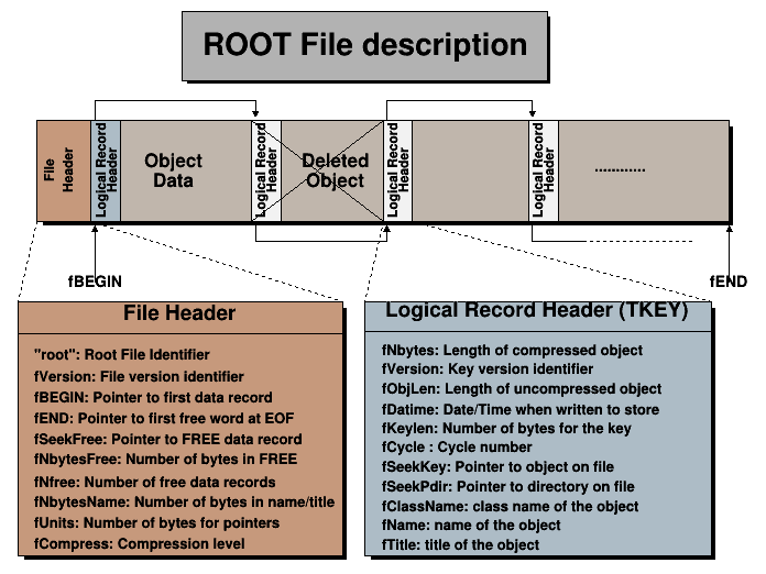
Figure 2.1: Description of the ROOT file physical format. ROOT
A ROOT file can contain unlimited levels of directories and objects, but the data of the ROOT objects is written in the file in consecutive order. In order to allow lookup on the object identifiers, the file header stores a pointer to the first element of the linked list of data objects’ logical records. Logically, this translates to keeping a hash list of entries (keys) for each directory and subdirectory (Figure 2.2). All this allows efficient sequential, random and hierarchical access to the data stored in the file.
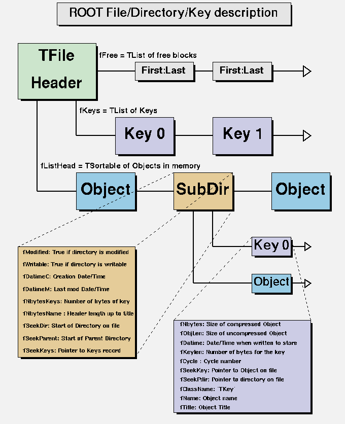
Figure 2.2: Description of the ROOT file logical format. ROOT
Finally, ROOT also considers data integrity when reading ROOT objects from a file written with a previous version of the framework. Because the description of all relevant classes is stored with the data, we need to support the evolution of the stored classes over the lifetime of a collaboration. For this purpose, ROOT will compare the versions of the persistified object and the object in memory, and automatically translate to the new format if possible. This feature is known as schema evolution.
All these features make the ROOT file format the most performant solution, both when reading and writing, compared to the most popular commercially available column-wise data storage formats8 9. This is in large part thanks to the TTree class.
2.2 The ROOT Trees#
TTree is the ROOT class optimized for I/O and memory usage. ROOT’s TTree represents a forest of Trees, each representing an entry, such as a specific event data, in the dataset. A ROOT Tree consists of branches and sub-branches, ultimately described by their leaves (data object). The leaves may be either complete objects of a class or individual data members of a given class, split as sub-branches of the same parent branch. This splitting process can be applied recursively, allowing for optimizations such as the grouping in branches of the data members of the different elements of a container. The optimal level of splitting depends on the tree’s usual access patterns, providing a great benefit in analyses where we only access few data members of the tree stored objects.
Splitting is especially useful for the (CWS) ROOT implements. By selectively reading the data needed at each moment, CWS reduces the volume of transferred data and I/O operations, improving dramatically the speed when gathering data. ROOT takes advantage of this by grouping in branches and storing contiguously the data elements frequently accessed together, optimizing random lookups to the data. This grouping, defined by the level of splitting, provides even higher benefits by applying further optimizations such as the parallel reading of the tree branches.
ROOT also implements several optimizations to improve writing accesses to memory, e.g. buffer writing; continuing with the analogy, when we gather the fruits (data) of a given branch, we collect them into baskets (buffers). When these baskets are full, we take them to the storage system (the file). This helps greatly reduce the number of (costly) accesses to disk.
However, given the nature of the data commonly processed by ROOT’s typical analyses, TTrees are usually too large to be practically stored in a single file, in terms of space, distribution or processing time. ROOT implements the class TChain for the reading of TTrees split in several TFiles, which abstracts the splitting from the user perspective. The storage of partitioned TTrees over several file facilitates the distribution of data in remote systems and the parallel and distributed processing of data analyses.
In addition, analyses usually access the same subset of branches for each one of the entries of a TTree. To dramatically improve this access, ROOT implements adaptative prefetching mechanisms, reading the following entry of the one being processed. This improves greatly the performance when processing remote ROOT files, making the bandwidth of the network, previously an important limiting factor, no longer a consideration.
3. Parallelism#
First developed in 1994—with segments of code dating up to a decade earlier—ROOT was already conceived with parallelism in mind. However, although considerable work was put into it by offering classes (TThread) and mechanisms for synchronization and mutual exclusion (e.g., TMutex or TCondition), this was not enough to meet the challenges posed by the ambitious LHC Physics program.
ROOT, a tool adopted by virtually all HEP experiments, needed to adapt to emerging hardware architectures but, while multiprocessing efforts were a success with the emergence of facilities such as , the multithreading efforts were hindered by early software architecture designs as they grew in ambition. These early designs were dependent on inherently non-thread-safe components, such as global variables or global bookkeeping and automatic garbage collection. In recent years, a greater allocation of manpower and other resources has enabled the deployment of multithreaded parallelism in a significant portion of the codebase, covering ROOT’s most performance-critical operations.
In this section we present some of the most relevant efforts in concurrent computing that ROOT has been focused on: PROOF, the parallel ROOT facility for distributed analysis (Section 3.1); the executors, a parallel implementation of the MapReduce pattern in ROOT (3.2); and the push in the user-oriented programming model, exemplified by the two modes of multithreaded execution of ROOT (Section 3.3): implicit and explicit execution modes, and vectorization (Section 3.4).
3.1 PROOF#
Multiprocessing in ROOT is particularly attractive because of its platform-independent streaming of C++ objects to disk, a feature that cannot be offered by any other multiprocessing framework. PROOF was a response to an increased demand for processing power at a time when the standard ROOT approach could not take advantage of the full processing capability of multi-core computers.
PROOF is an extension of ROOT that provides users with transparent, interactive multiprocess analysis over large remote datasets. PROOF is explicitly designed to work with the ROOT data stores and objects—such as the class used in ROOT for persistent event data, the TTree—relying on optimized initialization and traversing techniques, via the TSelector class.
The PROOF system is characterized by three properties: transparency, not requiring changes in the user programming model after set up; scalability, not limiting the number of processing units able to be used in parallel; and adaptability, being able to adapt itself to the changes in the remote environment. It presents a multi-tier architecture, its main components being the ROOT client sessions, the master node, and the slave nodes. In addition, it offers the possibility of executing physics analysis on a cluster of computers.
During the typical setup workflow of PROOF for a cluster, the user connects to the master node in the cluster, and the master node creates a slave server on each one of the nodes. In addition, we create a user space for each user of the system, where PROOF caches the packages and code used for the analysis and a temporary session log file. Each slave node, or worker, executes independently its own ROOT session, connecting the input and output streams of the command line interpreter to the network sockets. Once set up, the system is ready to process the physics analysis in a distributed, parallel, multi-processed fashion.
PROOF automatically takes care of synchronization, monitoring and scheduling, abstracting these complexities from the user. For better performance and load balancing, the analysis is split into small packages which will be assigned to the nodes on demand. The size of each package (the amount of work to process) depends on the characteristics (frequency, memory) of the client (slave) node.
Users program their analysis for PROOF as they would do for ROOT. PROOF was designed to support the programming models ROOT offered at the time for the expression of the analysis, namely by interacting with the GUI, programmatically via TSelectors and with TTDraw().
Although PROOF is currently kept in maintenance mode, it is still used in a considerable number of HEP experiments, and remains the only distributed analysis tool able to fully exploit ROOT capabilities. For example, at CHEP 201510, PROOF still featured in 7 of the presented proceedings for the conference.
Although PROOF provides a good solution for multi-node systems, due to the overhead that arises from the initialization and usage of its many components (which might not be necessary), it can exhibit suboptimal performance for analyses executed on local, single-node multicore hosts. For these analyses, PROOF might be replaced with PROOF-Lite 11, a lighter version of PROOF sharing the same programming model but offloading many components of PROOF which are not needed for single node execution (such as network connectivity). In addition, depending on the nature of the problem, users might benefit from using ROOT’s MapReduce facility for multi-process analysis in single node, TProcessExecutor12 (Section TProcessExecutor from the Task Level Parallelism in ROOT article), the multiprocess implementation of the executors’ programming model.
3.2 Executors: A new set of tools for expressing parallelism in ROOT#
It is often possible to identify repetitive tasks and frequently applied patterns or workflows in HEP analyses. Some of these patterns describe operations that are easy to express concurrently. ROOT exploits this idea by offering a parallel implementation of one of the most frequent patterns: MapReduce.
For this purpose, ROOT gathers inspiration from the Python concept of the executors, facilities that implement the MapReduce pattern in parallel. ROOT offers two executors, both of them implementing the interface defined by the parent class TExecutor:
-
TProcessExecutor: ROOT’s Multiprocess executor, a lighter multiprocessing framework than PROOF or PROOF-Lite, but limited to MapReduce operations. In addition to the executor interface, ROOT also extends TProcessExecutor functionalities with parallel processing and reading of ROOT trees.
-
TThreadExecutor: ROOT’s Multithreaded executor, built on top of the Intel TBB library. This executor offers chunking capabilities, NUMA awareness, parallel reduction and very low task overhead.
The executor model has proved to be successful and has been applied throughout ROOT as well as in standalone utilities such as hadd (see the hadd section in the Performance studies article of this series). It yields large speed up gains, especially in the most performance-critical operations, such as parallel reading of TTree branches (intra-event or inter-event) or parallel merging of buffers before writing. These executors are described in more detail in the article Task Level Parallelism in ROOT.
3.3 Implicit and explicit multithreading#
Parallel computing is usually considered challenging and complex, but it is unavoidable in today’s computer architectures when aiming for high performance.
One of the ways to overcome this complexity is to simplify the programming model. However, there is a tradeoff between giving users full control over the parallelization of the program, which requires at least basic knowledge of concepts such as threads, locks, or critical sections; and hiding the complexity from the user, which limits the parallelization to a certain set of predefined operations. Since version 6.12, ROOT offers both ways of expressing parallelism in a multithreaded way:
-
Explicit parallelism: users express parallelism explicitly, by working directly with the threading facilities of the C++ standard library; by using the libraries of their choice, such as TBB, Boost or OpenMP; or by abstracting the complexity by using the set of utilities for expressing parallelism ROOT provides.
-
Implicit parallelism: ROOT implicitly manages the concurrency in the user code, parallelizing expensive operations without requiring actions from the user.
Although ROOT also offers tools for the explicit expression of multithreaded parallelism, such as the executors, a great effort has been invested to adapt ROOT’s libraries to leverage implicit multithreading, and users are encouraged to prefer it over explicit parallelization. Nevertheless, the two options are not interface-exclusive, and, in some of the cases, for example when performing a fit (See section ), for user convenience, flexibility or interface coherency, both implicit and explicit parallelism are offered.
3.4 Vectorization#
ROOT implements parallelism at data-level by exploiting single instruction, multiple data (SIMD) vectorization. For this purpose, ROOT relies on three external libraries:
-
VDT is a mathematical library of fast implementations of transcendental functions automatically vectorizable by modern compilers. This includes the logarithm function, trigonometric functions and the inverse function.
-
Vc is a library designed to simplify the explicit expression of SIMD operations, offering a much more user-friendly programming model than the compiler intrinsics it is built on.
-
VecCore is a library that enables efficient vectorization by providing an abstraction layer on top of other vectorization libraries, such as Vc or UME::SIMD. This extra layer of abstraction facilitates the expression of SIMD operations in a user-friendly way. These libraries are supported as interchangeable backends along with a fallback scalar one, allowing the selection of the appropriate backend (e.g., the most efficient, the one that offers better support for the set of instructions available, etc.) for each specific architecture.
Although the three libraries can be built and enabled during the ROOT compilation process, VecCore is the only library explicitly used in ROOT, and enabling it allows users to benefit from features such as the new ROOT types relying on VecCore to perform SIMD operations; the support for functions built with these ROOT SIMD types in TF1 (Section TF1 in the Data-level parallelism in ROOT article); the vectorized evaluation of the fitting given a vectorized TF1 (see the Parallelization of the Fit in Root article of this series); or the compilation at runtime of vectorized functions thanks to TFormula (section TFormula section in the Performance studies article of this series).
4. Mathematical libraries#
Analyzing a large amount of complex data, such as that gathered by the LHC experiments, requires advanced mathematical and statistical computational methods. ROOT’s Math libraries13 are responsible for providing and supporting a coherent set of mathematical and statistical libraries required for simulation, reconstruction and analysis of High Energy Physics data.
These libraries are divided into several parts:
-
MathCore implements basic mathematical functions and algorithms commonly used in HEP data analysis, as well as a set of interfaces for its use and extension. They allow the user to plug-in at runtime different implementations of the numerical algorithms (e.g. different minimization algorithms when fitting), which are not required to co-exist in the same library (e.g., picking algorithms from ROOT’s MathMore library). MathCore includes utilities such as commonly used free functions, classes for random number generation, basic numerical algorithms (e.g., integration, derivation, minimization), and interfaces for defining function evaluation in one or more dimensions.
-
MathMore provides a more advanced collection of functions and interfaces for numerical computing. This library, an extension of MathCore that might be needed only for specific applications, wraps the GNU Scientific Library (GSL) and includes special mathematical functions, statistical and probabilistic functions present in GSL but not in MathCore, numerical algorithms from GSL, numerical integration and derivation classes, interpolation, function approximation using Chebysev polynomials, polynomial evaluation, and ROOT solvers.
-
The Linear Algebra libraries implement a complete environment for ROOT to perform calculations such as equation solving and eigenvalue decomposition, including the vector and matrix classes and linear algebra functions. ROOT implements its linear algebra operations in two libraries: a general matrix package (TMatrix in Figure 4.1) and an optimized one (SMatrix) for small and fixed-size matrices.
-
The fitting and minimization libraries provide classes and libraries that implement various fitting algorithms and function minimization methods. This includes both the classes and interfaces under the namespace Fit in ROOT and RooFit, used for fitting of probabilistic distributions (Sections 4.1 and 4.2respectively), and the various minimization libraries (minimizers) supported by ROOT for different minimization algorithms. These minimizers are distributed, depending on their usage, throughout ROOT math libraries, i.e. in MathCore, such as Minuit 2 or Fumili, or in MathMore, such as the minimizers from the GSL.
-
The Statistical libraries are mostly composed of libraries that implement machine learning and multivariate analysis methods (TMVA) and advanced statistical tools for computing confidence levels and discovery significances (RooStats, Section 4.2).
-
The Histogram library is used for displaying and analyzing one-dimensional or multidimensional binned data. Histograms are the most common way of representing the large amounts of data gathered in HEP experiments, as they reduce the complexity of the computations several fold without necessarily reducing their accuracy or significance in a considerable way. This library also contains the bounded function class in ROOT, TF1, which is fundamental for most of the mathematical operations in the libraries mentioned above.
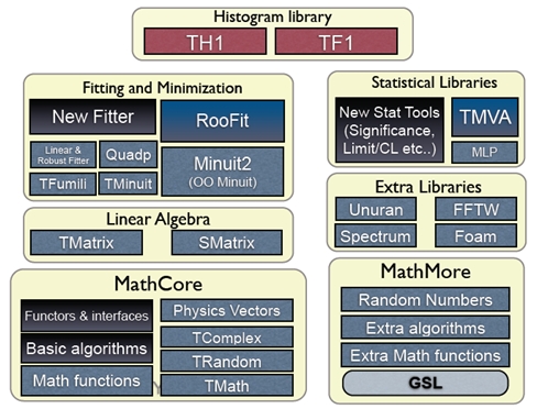
Figure 4.1: Math libraries and packages in ROOT.
4.1. Fitting#
ROOT provides several techniques for fitting14 that are applied depending on the user’s choice or type of data (differentiating between binned and unbinned data). These techniques, most of which are described in the Fitting fundamentals section of the Parallelization of ROOT fitting classes article, include methods such as the maximum likelihood method, applied for unbinned datasets; the least squares method, applied for binned datasets; or the Poisson likelihood method, applied for Poisson-described binned datasets.
The implementation of ROOT’s fitting process is highly modular, and it is composed of five main components: the user function model, the fitting data, the fitting method, the fitter and the minimizer.
The signature of the model function provided by the user should be compatible with the parametric function interface callable operator in ROOT, and it is provided via a function class in ROOT, e.g. TF1. To allow that the fitting method function classes interface with it, the ROOT class representing the model function needs to be wrapped in a class that implements the parametric function interface. The type of the data to fit, also specified by the user, is identified and described either with the unbinned data or the binned data class representations that ROOT implements. The appropriate objective function class is then built with the wrapped parametric function class object and the fit data representations.
The fitter is the class that manages the fitting process and interfaces the objective function with the minimizer class. It is also responsible for setting all the control parameters and options of the fit, such as allowing the selection of the appropriate minimization algorithm at runtime depending on the complexity of the problem.
ROOT implements interfaces to several minimization algorithms and classes: numerical minimizers, such as Minuit, Minuit2 and Fumili; stochastic minimizers, such as the GSL minimizer based on simulated annealing; and even minimizers based on genetic algorithms.
This modular design allows the reusability of the model, e.g. with different types of data sets or functions, but increases the overall complexity of the process. ROOT provides a way to hide this complexity from the user: calling the fitting process via the Fit method implemented on the most important ROOT object classes, such as histograms, graphs and trees (Listing 4.1, Figure 4.2). More information about the fitting, as well as the modifications implemented to parallelize the fitting process, both at task-level and at data-level, are provided in the article Parallelization of the Fit in Root.
 std::unique_ptr<TF1> f1("f1", "gaus");
 f1->SetParameters(1, 0, 1);

 h1->Fit(f1);
Listing 4.1: Fitting of the histogram h1 with a Gaussian function in ROOT by calling its member function Fit.
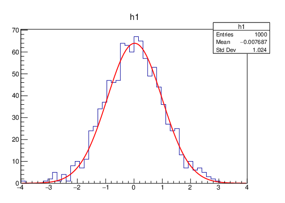
Figure 4.2: Plot result automatically obtained when fitting a histogram with a Gaussian function in ROOT as shown in Listing 4.1.
4.2 RooFit and RooStats#
ROOT mathematical libraries provide a set of methods, functions and libraries that respond to the needs of the majority of traditional HEP experiments and analyses. However, the LHC experiments demand more powerful advanced fitting and advanced statistical functionality for some of their analyses. For these cases, ROOT distributes with it the RooFit and RooStats packages.
RooFit15 is a library that allows building more complex models than ROOT’s fitting, e.g. combining probability density functions; performing fits, e.g. maximum likelihood, and generating its respective plots; and generating Monte Carlo samples. It is also oriented to large-scale projects. RooFit was designed to be used with ROOT, and it delegates important parts of the underlying functionality to ROOT when possible.
RooStats16 is a library that extends ROOT functionality with advanced statistical tools, with emphasis on discovery significance, hypothesis testing, confidence intervals, and combined measurements. These tools, based on the RooFit classes for describing probability density functions or likelihood functions, aim to satisfy the requirements of the LHC experiments and, therefore, include the major statistical techniques approved by the Experiment Statistical Committee to perform the aforementioned measurements.
5. RDataFrame#
RDataFrame is a programming paradigm available in ROOT that allows its users to express their analyses declaratively in a functional way.
RDataFrame entails a paradigm shift in the way HEP analyses are expressed. By renouncing full control of the event loop, an iterative process over the data recorded from collisions, the user obtains something potentially more powerful: complete control over the expression of the analysis; that is to say, instead of investing time and effort in designing and implementing the details of the analysis computation, the user specifies the different operations that compose the analysis while the framework manages the underlying complexity and optimizations.
RDataFrame hides the complexity of the TTree and the branch-based columnar storage by reasoning in terms of entries and columns. A RDataFrame analysis is composed of actions, such as creating and filling a histogram or computing the mean of the values of a column (a branch in the tree structure of Section TTree), and of transformations, e.g. filtering data or creating new columns. These operations are combined and pipelined by connecting them in functional chains. Listing 5.1 compares the traditional way (lines 2-7) of filling a histogram with the entries that pass the IsGoodEntry filter against the same operation expressed with RDataFrame ((lines 11-12), showcasing the chaining of actions and transformations.
// Traditional programming model
TTreeReader reader(data);
TTreeReaderValue<A> x(reader,"x");
TTreeReaderValue<B> y(reader,"y");
TTreeReaderValue<C> z(reader,"z");
while (reader.Next()) {
   if (IsGoodEntry(*x, *y, *z)) {
      h->Fill(*x);
   }
}

// RDataFrame
RDataFrame d(data);
auto h = d.Filter(IsGoodEntry, {"x","y","z"}).Histo1D("x");
Listing 5.1: Comparison of the traditional programming model against RDataFrame.
While the functional chains were the original idea that sparked the implementation of RDataFrame, it soon became clear that it was more beneficial to express the analysis as a computational graph. Expressing the analysis by means of functional chains requires us to execute all actions and transformations in a single loop over all entries. In addition, expressing it in terms of a functional graph allows us to potentially increase the benefits obtained from a lazy execution of the loop: the loop is executed when accessing an end node of the graph or chain, another feature of RDataFrame. That is to say, given several end nodes of the graph, the loop will be executed only once for their shared actions and transformations, rather than evaluating the whole loop for each functional chain. Section nuon in the Performance Studies article from this series details this lazy evaluation, providing an example of a functional graph.
These optimizations of the functional graph require the user to delegate control of the event loop to RDataFrame. Traditional approaches offer more detail and customization possibilities for the computation of the loop, at the cost of increased complexity, unavoidable boilerplate code, and non-trivial parallelization. Instead, RDataFrame emphasizes the programming model, by offering high-level features such as better expressivity, language economy and, most importantly, the abstraction of complex operations, e.g. developing parallel code.
// Traditional programming model
TTreeReader reader(data);
TTreeReaderValue<A> x(reader,"x");
TTreeReaderValue<B> y(reader,"y");
TTreeReaderValue<C> z(reader,"z");
while (reader.Next()) {
   if (IsGoodEntry(*x, *y, *z)) {
      h->Fill(*x);
   }
}

// RDataFrame
RDataFrame d(data);
auto h = d.Filter(IsGoodEntry, {"x","y","z"}).Histo1D("x");
Listing 5.2: Comparison of the compact and fully expressive formulation of a RDataFrame analysis.
Thanks to Cling, we can further simplify the programming model, improving the expressivity and economy of the language by JIT-compiling, translating simplified user interfaces into fully templated code at runtime. Listing 5.2 showcases two formulations of the same expression. While both are available, it is usually more convenient for the user to leverage the compact formulation (lines 11-12), at the cost of including minimal overhead by the runtime compilation.
Parallelization is built in at the core of RDataFrame, handled through the implicit multithreading (Section 3.3) mechanisms of ROOT, and will be employed when possible, from the parallelization of the event loop at entry level to the parallel writing of the data frame on disk.
RDataFrame works not only with the ROOT format but with others as popular and important as CSV and Apache Arrow17, providing an adapter to read and convert these formats into the ROOT format.
RDataFrame’s implementation respects modern C++ best practices and aggressively adopts template metaprogramming, which allows it to benefit from improvements such as the absence of virtual calls or type-safe access to the datasets. In addition, ROOT’s Python library, PyROOT, has been considered during each stage of the design of RDataFrame, in order to provide seamless integration that paves the way for the interaction with some of the (currently) most important data science libraries, such as NumPy18, Pandas19 or TensorFlow20.
All the benefits obtained from RDataFrame’s declarative programming model, along with the exceptional performance exhibited, triggers its fast adoption by HEP’s most important experiments.
The nuon section in the Performance Studies article describes how by porting a highly optimized, ad-hoc, parallel code to RDataFrame we can not only match the speed up gains obtained by the original analysis but also improve scaling both in commodity laptops and massive parallel architectures.
6. User Interfaces and visualization#
One of the most important features of ROOT, together with the interpreter and the highly performant I/O, the one responsible for ROOT’s fast adoption by the community, is the development of a comprehensive set of visualization tools for HEP data analysis results and objects.
For simplicity and fast exploration of the results, any class inheriting from TObject has a Draw method, which will generate a graphical representation of the caller object in a ROOT canvas, the area mapped to a system graphical window. This automatically-generated graphical representation is implemented as well in most of the ROOT methods generating end results, such as the method of a histogram.
In addition, users may request full control over the graphical representation of their results, either for customization or to improve the default visualization. For this purpose, ROOT allows the user to define and generate the components of a plot programmatically, exposing all the different components of the visualization in a set of classes and, therefore, providing high customization and configuration of the graphic results (e.g. Figure 6.1). This is especially useful in combination with the interpreter, whose interactivity and visibility into the state of a program is ideal for the exploration and development of incremental improvements.
Figure 6.2 showcases some of the graphical representations, both in 2D and 3D, available in ROOT.
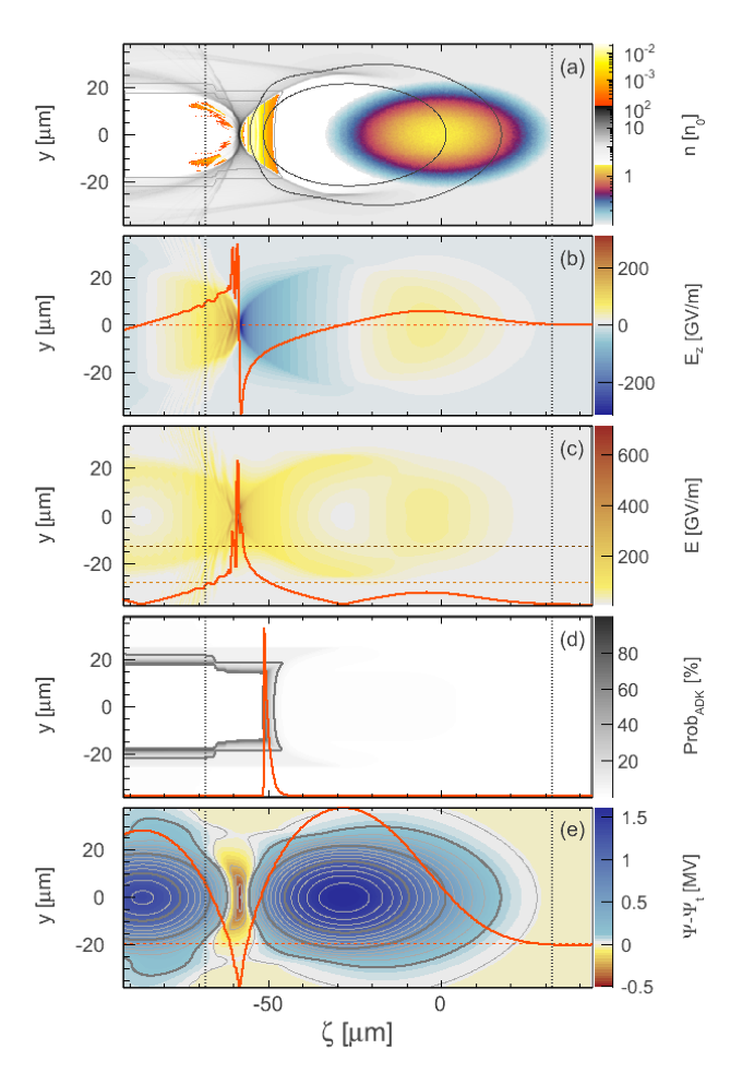
Figure 6.1:Example of how color palettes and transparency can be combined in ROOT. ROOT
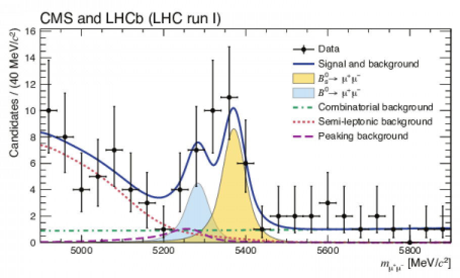
(a): Observation of the rare B0 s → µ+µ− decay from the combined analysis of CMS and LHCb data. ROOT gallery
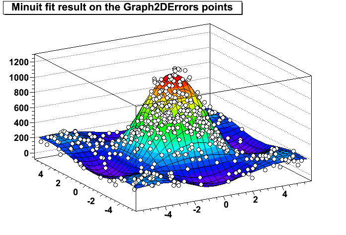
(b): Minuit fit result on the Graph2DErrors points. ROOT gallery
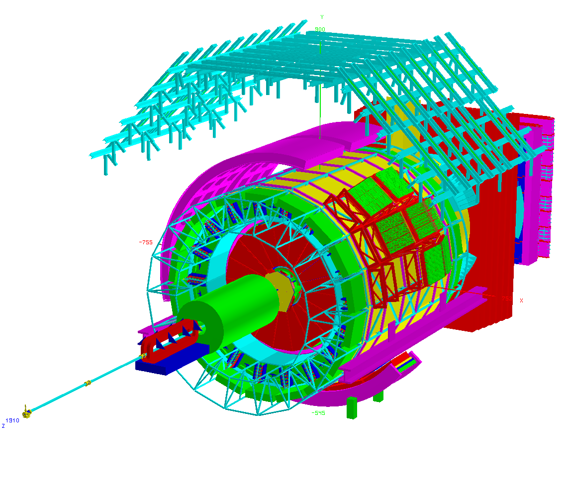
(c): 3D plot of the ALICE detector. ROOT gallery
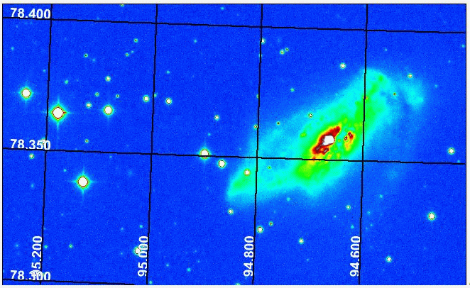
(d): Astrophysics example. ROOT gallery
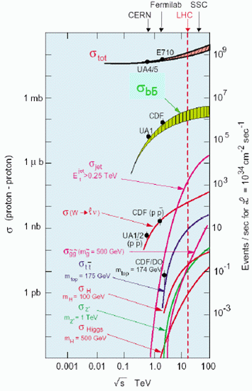
(e): Cross-sections vs. centre-of-mass energy for proton-proton interactions. ROOT gallery
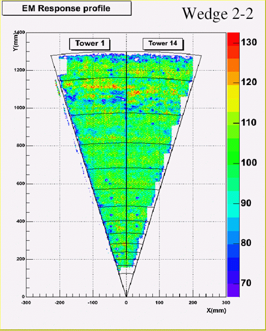
(f): Electromagnetic response. ROOT gallery
Figure 6.2: Showcase of some of the plots available in the ROOT graphics package.
6.1 The Graphical User Interface#
ROOT is distributed with a Graphical User Interface (GUI), a user-friendly way to interact with ROOT objects that is very rich in features, offering real-time interactivity and modification of the components of a canvas (possible thanks to the interactive interpreter); automatic generation of the C++ source code for the modified objects; and exploration of the contents of a ROOT file. Figure 6.3 showcases the different context menus obtained when selecting different components on a ROOT canvas, and the actions allowed on them directly accessible through the GUI, without writing code.
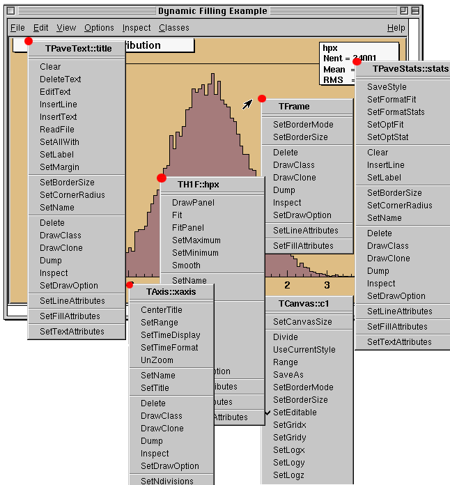
Figure 6.3: Context menus for the objects drawn on the ROOT canvas. ROOT user’s guide
ROOT also offers a development toolkit, the ROOT GUI builder, a set of ROOT classes used to develop internal components of the GUI. This includes context menus, the fit panel (Figure 6.4) or the TBrowser, a class for browsing ROOT files. The ROOT GUI builder is also used to develop external applications, such as event displays (Figure 6.5) or experiment-specific visualization tools, e.g. AliEVE21.
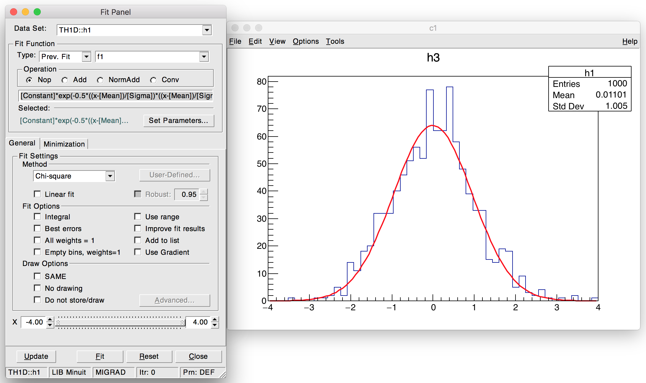
Figure 6.4: The fit panel.
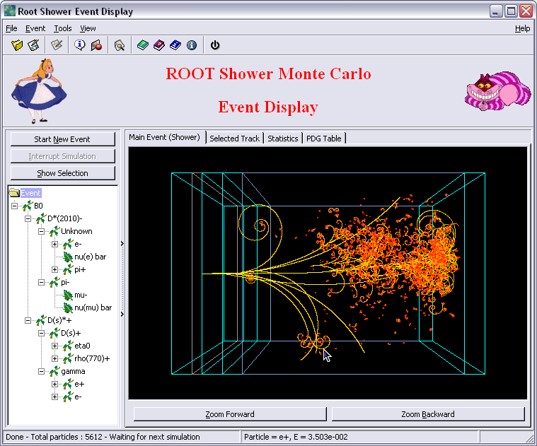
Figure 6.5: Shower Monte Carlo event display built with the ROOT GUI Builder. ROOT gallery
-
Rene Brun and Fons Rademakers. Root - an object oriented data analysis framework. In Nucl. Inst. and Meth. in Phys., editors, Proceedings AIHENP’96 Workshop, volume A389, pages 81–86, January 1997. link ↩︎
-
Enrico Guiraud, Axel Naumann, & Danilo Piparo. (2017, January 27). TDataFrame: functional chains for ROOT data analyses (Version v1.0). Zenodo. link ↩︎
-
Danilo Piparo, Enric Tejedor, Pere Mato, Luca Mascetti, Jakub Moscicki, and Massimo Lamanna. SWAN: A service for interactive analysis in the cloud. Future Generation Computer Systems, 78:1071–1078, 2018. [link] (https://cds.cern.ch/record/2158559) ↩︎
-
Rapid application development: https://en.wikipedia.org/wiki/Rapid_application_development ↩︎
-
Read-eval-print-loop: https://en.wikipedia.org/wiki/Read%E2%80%93eval%E2%80%93print_loop ↩︎
-
V Vasilev, P Canal, A Naumann, and P Russo. Cling–the new interactive interpreter for root 6. In Journal of Physics: Conference Series, volume 396, page 052071. IOP Publishing, 2012. ↩︎
-
Brian Bockelman, Oksana Shadura. Zstd & lz4. https://indico.fnal.gov/event/16264/contribution/8/material/slides/0.pdf ↩︎
-
Jim Pivarski. Parquet data format performance. https://indico.fnal.gov/event/16264/contribution/1/material/slides/0.pdf ↩︎
-
Jakob Blomer. A quantitative review of data formats for hep analyses. In Journal of Physics: Conference Series (Vol. 1085, No. 3, p. 032020). IOP Publishing, 2018. link ↩︎
-
H Sakamoto, D Bonacorsi, I Ueda, and A Lyon. 21st international conference on computing in high energy and nuclear physics (chep2015). Journal of Physics: Conference Series, 664(00):001001, 2015. ↩︎
-
C Aguado-Sanchez, J Blomer, P Buncic, I Charalampidis, G Ganis, M Nabozny, and F Rademakers. Studying root i/o performance with proof-lite. In Journal of Physics: Conference Series, volume 331, page 032010. IOP Publishing, 2011. link ↩︎
-
Guiraud, E., & Ganis, G. (2015, September 1). Enhancements to Multiprocessing in ROOT. Zenodo. link ↩︎
-
Moneta, L., Antcheva, I., & Brun, R. (2008). Recent developments of the ROOT mathematical and statistical software. In Journal of Physics: Conference Series (Vol. 119, No. 4, p. 042023). IOP Publishing. link ↩︎
-
Lorenzo Moneta, I Antcheva, and D Gonzalez Maline. Recent improvements of the root fitting and minimization classes. PoS, page 075, 2008. link ↩︎
-
Wouter Verkerke and David Kirkby. The roofit toolkit for data modeling. In Statistical Problems in Particle Physics, Astrophysics and Cosmology, pages 186–189. World Scientific, 2006 link ↩︎
-
Moneta, L., Belasco, K., Cranmer, K., Kreiss, S., Lazzaro, A., Piparo, D., … & Wolf, M. (2010). The roostats project. link ↩︎
-
Apache arrow: https://arrow.apache.org/ ↩︎
-
Numpy: http://www.numpy.org/ ↩︎
-
Wes McKinney. Data structures for statistical computing in python. In Stéfan van der Walt and Jarrod Millman, editors, Proceedings of the 9th Python in Science Conference, pages 51 – 56, 2010 link ↩︎
-
Martin Abadi, Paul Barham, Jianmin Chen, Zhifeng Chen, Andy Davis, Jeffrey Dean, Matthieu Devin, Sanjay Ghemawat, Geoffrey Irving, Michael Isard, Manjunath Kudlur, Josh Levenberg, Rajat Monga, Sherry Moore, Derek G. Murray, Benoit Steiner, Paul Tucker, Vijay Vasudevan, Pete Warden, Martin Wicke, Yuan Yu, and Xiaoqiang Zheng. Tensorflow: A system for large-scale machine learning. In 12th USENIX Symposium on Operating Systems Design and Implementation (OSDI 16), pages 265–283, 2016. link ↩︎
-
Matevz Tadel et al. Alieve-alice event visualization environment link ↩︎